
Version info: Code for this page was tested in Stata 12.
Zero-inflated poisson regression is used to model count data that has an excess of zero counts.
Further, theory suggests that the excess zeros
are generated by a separate process from the count values and that the excess zeros can
be modeled independently. Thus, the zip model has two parts, a
poisson count model and the logit model
for predicting excess zeros. You may want to review these Data Analysis Example pages,
Poisson Regression and
Logit Regression.
Please Note: The purpose of this page is to show how to use various data analysis commands.
It does not cover all aspects of the research process which researchers are expected to do. In
particular, it does not cover data cleaning and verification, verification of assumptions, model
diagnostics and potential follow-up analyses.
Examples of zero-inflated Poisson regression
Example 1.
School administrators study the attendance behavior of high school juniors over
one semester at two schools. Attendance is measured by number of days of
absent and is predicted by gender of the student and standardized
test scores in math and language arts. Many students have no absences
during the semester.
Example 2.
The state wildlife biologists want to model how many fish are being caught by fishermen
at a state park. Visitors are asked whether or not they have a camper, how many
people were in the group, were there children in the group and how many fish were caught.
Some visitors do not fish, but there is no data on whether a person fished or not. Some
visitors who did fish did not catch any fish so there are excess zeros in the data because
of the people that did not fish.
Description of the data
Let’s pursue Example 2 from above.
We have data on 250 groups that went to a park. Each group was questioned
about how many fish they caught (count), how many children were in the
group (child), how many people were in the group (persons), and
whether or not they brought a camper to the park (camper).
In addition to predicting the number of fish caught, there is interest in
predicting the existence of excess zeros, i.e. the zeroes that were not simply a
result of bad luck fishing. We will use the variables child, persons, and
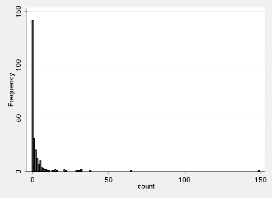
camper in our model. Let’s look at the data.
use http://www.stata-press.com/data/r10/fish, clear
summarize count child persons camper
Variable | Obs Mean Std. Dev. Min Max
-------------+--------------------------------------------------------
count | 250 3.296 11.63503 0 149
child | 250 .684 .8503153 0 3
persons | 250 2.528 1.11273 1 4
camper | 250 .588 .4931824 0 1
histogram count, discrete freq
 tab1 child persons camper
-> tabulation of child
child | Freq. Percent Cum.
------------+-----------------------------------
0 | 132 52.80 52.80
1 | 75 30.00 82.80
2 | 33 13.20 96.00
3 | 10 4.00 100.00
------------+-----------------------------------
Total | 250 100.00
-> tabulation of persons
persons | Freq. Percent Cum.
------------+-----------------------------------
1 | 57 22.80 22.80
2 | 70 28.00 50.80
3 | 57 22.80 73.60
4 | 66 26.40 100.00
------------+-----------------------------------
Total | 250 100.00
-> tabulation of camper
camper | Freq. Percent Cum.
------------+-----------------------------------
0 | 103 41.20 41.20
1 | 147 58.80 100.00
------------+-----------------------------------
Total | 250 100.00
tab1 child persons camper
-> tabulation of child
child | Freq. Percent Cum.
------------+-----------------------------------
0 | 132 52.80 52.80
1 | 75 30.00 82.80
2 | 33 13.20 96.00
3 | 10 4.00 100.00
------------+-----------------------------------
Total | 250 100.00
-> tabulation of persons
persons | Freq. Percent Cum.
------------+-----------------------------------
1 | 57 22.80 22.80
2 | 70 28.00 50.80
3 | 57 22.80 73.60
4 | 66 26.40 100.00
------------+-----------------------------------
Total | 250 100.00
-> tabulation of camper
camper | Freq. Percent Cum.
------------+-----------------------------------
0 | 103 41.20 41.20
1 | 147 58.80 100.00
------------+-----------------------------------
Total | 250 100.00
Analysis methods you might consider
Below is a list of some analysis methods you may have encountered.
Some of the methods listed are quite reasonable while others have either fallen out of favor or
have limitations.
- Zero-inflated Poisson Regression – The focus of this web page.
- Zero-inflated Negative Binomial Regression – Negative binomial regression does better with
over dispersed data, i.e. variance much larger than the mean. - Ordinary Count Models – Poisson or negative binomial models might be more
appropriate if there are no excess zeros. - OLS Regression – You could try to analyze these data using OLS regression. However, count
data are highly non-normal and are not well estimated by OLS regression.
Zero-inflated Poisson regression
We will run the zip command with child and camper as predictors of the counts,
persons as the predictor of the excess zeros.
zip count child camper, inflate(persons)

Fitting constant-only model:

Iteration 0:   log likelihood =  -1347.807
Iteration 1:   log likelihood = -1315.5343
Iteration 2:   log likelihood = -1126.3689
Iteration 3:   log likelihood = -1125.5358
Iteration 4:   log likelihood = -1125.5357
Iteration 5:   log likelihood = -1125.5357

Fitting full model:

Iteration 0:   log likelihood = -1125.5357
Iteration 1:   log likelihood = -1044.8553
Iteration 2:   log likelihood = -1031.8733
Iteration 3:   log likelihood = -1031.6089
Iteration 4:   log likelihood = -1031.6084
Iteration 5:   log likelihood = -1031.6084

Zero-inflated Poisson regression                  Number of obs   =        250
                                                  Nonzero obs     =        108
                                                  Zero obs        =        142

Inflation model = logit                           LR chi2(2)      =     187.85
Log likelihood  = -1031.608                       Prob > chi2     =     0.0000

------------------------------------------------------------------------------
       count |      Coef.   Std. Err.      z    P>|z|     [95% Conf. Interval]
-------------+----------------------------------------------------------------
count        |
       child |  -1.042838   .0999883   -10.43   0.000    -1.238812    -.846865
    1.camper |   .8340222   .0936268     8.91   0.000      .650517    1.017527
       _cons |   1.597889   .0855382    18.68   0.000     1.430237     1.76554
-------------+----------------------------------------------------------------
inflate      |
     persons |  -.5643472   .1629638    -3.46   0.001    -.8837503    -.244944
       _cons |   1.297439   .3738522     3.47   0.001     .5647022    2.030176
------------------------------------------------------------------------------
The output looks very much like the output from an OLS regression:
-
- Begins with
the iteration log giving the values of the log likelihoods starting
with a constant-only model that has no predictors for the count model and the intercept only sets to zero for the inflated model. Then the second part, fitting full model, starts with estimated parameters for the inflated model and intercept only model for the count model until iteration converges to estimation of the full model. The last value in the log is the final value
of the log likelihood for the full model and is repeated below. - Next comes the header information. On the right-hand side the number of
observations used (250), number of nonzero observations (108) are given along with the likelihood
ratio chi-squared.
This compares the full model to a model without count predictors, giving a
difference of two degrees of freedom. This is followed by the p-value for
the chi-square. The model, as a whole, is statistically significant. - Below the header you will find the Poisson regression coefficients for each of the
count predicting variables
along with standard errors, z-scores, p-values and 95% confidence intervals for the
coefficients. - Following these are logit coefficients for the variable predicting excess zeros along
with its standard errors, z-scores, p-values and confidence intervals.
- Begins with
Cameron and Trivedi (2009) recommend robust standard errors for Poisson models.
We will rerun the model with the vce(robust) option.
zip count child i.camper, inflate(persons) vce(robust)

Fitting constant-only model:

Iteration 0:   log pseudolikelihood =  -1347.807
Iteration 1:   log pseudolikelihood = -1315.5343
Iteration 2:   log pseudolikelihood = -1126.3689
Iteration 3:   log pseudolikelihood = -1125.5358
Iteration 4:   log pseudolikelihood = -1125.5357
Iteration 5:   log pseudolikelihood = -1125.5357

Fitting full model:

Iteration 0:   log pseudolikelihood = -1125.5357
Iteration 1:   log pseudolikelihood = -1044.8553
Iteration 2:   log pseudolikelihood = -1031.8733
Iteration 3:   log pseudolikelihood = -1031.6089
Iteration 4:   log pseudolikelihood = -1031.6084
Iteration 5:   log pseudolikelihood = -1031.6084

Zero-inflated Poisson regression                  Number of obs   =        250
                                                  Nonzero obs     =        108
                                                  Zero obs        =        142

Inflation model      = logit                      Wald chi2(2)    =       7.25
Log pseudolikelihood = -1031.608                  Prob > chi2     =     0.0266

------------------------------------------------------------------------------
             |               Robust
       count |      Coef.   Std. Err.      z    P>|z|     [95% Conf. Interval]
-------------+----------------------------------------------------------------
count        |
       child |  -1.042838   .3893772    -2.68   0.007    -1.806004   -.2796731
    1.camper |   .8340222   .4076029     2.05   0.041     .0351352    1.632909
       _cons |   1.597889   .2934631     5.44   0.000     1.022711    2.173066
-------------+----------------------------------------------------------------
inflate      |
     persons |  -.5643472   .2888849    -1.95   0.051    -1.130551    .0018567
       _cons |   1.297439    .493986     2.63   0.009     .3292445    2.265634
------------------------------------------------------------------------------
Now we can move on to the specifics of the individual results.
- Using the robust option has resulted in a fairly large change in the model chi-square,
which is now a Wald chi-square. This statistic is based on log pseudo-likelihoods instead of
log-likelihoods. - The coefficients for child and camper can be interpreted as follows:
- For each unit increase of child the expected log count of the response variable decreases by 1.043.
- Being a camper increases the expected log count by .834.
- The inflate coefficient for persons
suggests that for each unit increase in person the log odds of an inflated zero decrease by
.564.
We can use the margins to help understand our model. We will
first compute the expected counts for the categorical variable camper while holding the
continuous variable child at its mean value using the atmeans option.
margins camper, atmeans

Adjusted predictions                              Number of obs   =        250
Model VCE    : Robust

Expression   : Predicted number of events, predict()
at           : child           =        .684 (mean)
               0.camper        =        .412 (mean)
               1.camper        =        .588 (mean)
               persons         =       2.528 (mean)

------------------------------------------------------------------------------
             |            Delta-method
             |     Margin   Std. Err.      z    P>|z|     [95% Conf. Interval]
-------------+----------------------------------------------------------------
      camper |
          0  |   1.289132   .4393168     2.93   0.003     .4280866    2.150177
          1  |   2.968305    .619339     4.79   0.000     1.754423    4.182187
------------------------------------------------------------------------------
The expected count for the number of fish caught by non-campers is 1.289 while for campers it is
2.968 at the means of child and persons.
Using the dydx option computes the difference in expected counts between camper
= 0 and camper = 1 while still holding child at its mean of .684
and persons at its mean of 2.528.
margins, dydx(camper) atmeans

Conditional marginal effects                      Number of obs   =        250
Model VCE    : Robust

Expression   : Predicted number of events, predict()
dy/dx w.r.t. : 1.camper
at           : child           =        .684 (mean)
               0.camper        =        .412 (mean)
               1.camper        =        .588 (mean)
               persons         =       2.528 (mean)

------------------------------------------------------------------------------
             |            Delta-method
             |      dy/dx   Std. Err.      z    P>|z|     [95% Conf. Interval]
-------------+----------------------------------------------------------------
    1.camper |   1.679173   .7754611     2.17   0.030     .1592975    3.199049
------------------------------------------------------------------------------
Note: dy/dx for factor levels is the discrete change from the base level.
The difference in the number of fish caught by campers and non-campers is 1.679, which is
statistically significant.
One last margins command will give the expected counts for values of child
from zero to three at both levels of camper.
margins, at(child=(0(1)3) camper=(0/1)) vsquish


Predictive margins                                Number of obs   =        250
Model VCE    : Robust

Expression   : Predicted number of events, predict()
1._at        : child           =           0
               camper          =           0
2._at        : child           =           0
               camper          =           1
3._at        : child           =           1
               camper          =           0
4._at        : child           =           1
               camper          =           1
5._at        : child           =           2
               camper          =           0
6._at        : child           =           2
               camper          =           1
7._at        : child           =           3
               camper          =           0
8._at        : child           =           3
               camper          =           1

------------------------------------------------------------------------------
             |            Delta-method
             |     Margin   Std. Err.      z    P>|z|     [95% Conf. Interval]
-------------+----------------------------------------------------------------
         _at |
          1  |   2.616441   .6470522     4.04   0.000     1.348242     3.88464
          2  |   6.024516   2.159288     2.79   0.005      1.79239    10.25664
          3  |    .922172   .4142303     2.23   0.026     .1102954    1.734048
          4  |   2.123358   .4771534     4.45   0.000     1.188154    3.058561
          5  |   .3250221   .2611556     1.24   0.213    -.1868335    .8368777
          6  |   .7483834   .3929987     1.90   0.057    -.0218798    1.518647
          7  |    .114555   .1351887     0.85   0.397    -.1504101      .37952
          8  |   .2637699   .2365495     1.12   0.265    -.1998587    .7273984
------------------------------------------------------------------------------

marginsplot
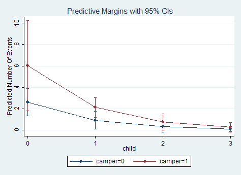
The expected number of fish caught goes down as the number of children goes up
for both people with and without campers.
A number of model fit indicators are available using the fitstat command, which is
part of the spostado utilities by J. Scott Long and Jeremy Freese (search spostado).
fitstat

Measures of Fit for zip of count

Log-Lik Intercept Only:      -1127.023   Log-Lik Full Model:          -1031.608
D(244):                       2063.217   LR(4):                         190.829
                                         Prob > LR:                       0.000
McFadden's R2:                   0.085   McFadden's Adj R2:               0.079
ML (Cox-Snell) R2:               0.534   Cragg-Uhler(Nagelkerke) R2:      0.534
AIC:                             8.301   AIC*n:                        2075.217
BIC:                           715.980   BIC':                         -168.743
BIC used by Stata:            2090.824   AIC used by Stata:            2073.217
Things to consider
- Since zip has both a count model and a logit
model, each of the two models should have good predictors. The two models do not
necessarily need to use the same predictors. - Problems of perfect prediction, separation or partial separation can occur in the
logistic part of the zero-inflated model. - Count data often use exposure variables to indicate the number of times the event
could have happened. You can incorporate exposure into your model by using the exposure()
option. - It is not recommended that zero-inflated Poisson models be applied to
small samples. What constitutes a small sample does not seem to be clearly defined
in the literature. - Pseudo-R-squared values differ from OLS R-squareds, please see
FAQ: What are
pseudo R-squareds? for a discussion on this issue. - In times past, the Vuong test had been used to test whether a zero-inflated Poisson model or a Poisson model (without the zero-inflation) was a better fit for the data. However, this test is no longer considered valid. Please see The Misuse of The Vuong Test For Non-Nested Models to Test for Zero-Inflation by Paul Wilson for further information.
See also
References
- Cameron, A. Colin and Trivedi, P.K. (2009) Microeconometrics using stata. College Station, TX: Stata
Press. - Long, J. Scott, & Freese, Jeremy (2006). Regression Models for Categorical Dependent Variables
Using Stata (Second Edition). College Station, TX: Stata Press. - Long, J. Scott (1997). Regression Models for Categorical and Limited Dependent Variables.
Thousand Oaks, CA: Sage Publications.