
SAS code file for live presentation (right-click to download)
Dataset used with code file (click on “DEMO_G_Data [XPT – 3.6MB]” to download; Note: this dataset is not the same as the dataset used for the webpage below)
The purpose of this workshop is to explore some issues in the analysis of
survey data using SAS 9.44 and SAS/Stat 15.2. Most of code shown in this
seminar will work in earlier versions of SAS and SAS/Stat. To find out
what version of SAS and SAS/Stat you are running, open SAS and look at the
information in the log file.
NOTE: SAS (r) Proprietary Software 9.4 (TS1M7)

NOTE: Updated analytical products:

      SAS/STAT 15.2
      SAS/ETS 15.2
      SAS/OR 15.2
      SAS/IML 15.2
      SAS/QC 15.2
There are seven survey procedures.
proc surveyselect: This procedure can be used to select a sample
from a dataset.
proc surveyimpute: This procedure can be used to do single imputations on a survey dataset.
proc surveymeans: This procedure can be used to obtain weighted
descriptive statistics for continuous variables. This procedure can produce graphs.
proc surveyfreq: This procedure can be used to run weighted one-way and
multi-way crosstabulations. This procedure can produce graphs.
proc surveyregress: This procedure can be used to run weighted
OLS regressions.
proc surveylogistic: This procedure can be used to run weighted
logistic, ordinal, multinomial and probit regressions.
proc surveyphreg: This procedure can be used to run weighted proportional
hazards regression.
We will also briefly discuss proc glimmix.
proc glimmix: This procedure will allow for sampling weights, so
it can be used to run weighted multilevel models. This procedure does not
have a strata, cluster or a domain statement, and it does not
allow for replicate weights. It requires that a sampling weight be specified at each level of the model.
Why do we need survey data analysis software?
Regular statistical software (that is not designed for survey data) analyzes
data as if the data were collected using simple random sampling. For
experimental and quasi-experimental designs, this is exactly what we want.
However, very few surveys use a simple random sample to collect data. Not only
is it nearly impossible to do so, but it is not as efficient (either financially
and statistically) as other sampling methods. When any sampling method other
than simple random sampling is used, we usually need to use survey data analysis
software to take into account the differences between the design that was used
to collect the data and simple random sampling. This is because the sampling
design affects both the calculation of the point estimates and the standard
errors of those estimates. If you ignore the sampling design, e.g., if you
assume simple random sampling when another type of sampling design was used,
both the point estimates and their standard errors will likely be calculated
incorrectly. The sampling weight will affect the calculation of the point
estimate, and the stratification and/or clustering will affect the calculation
of the standard errors. Ignoring the clustering will likely lead to standard
errors that are underestimated, possibly leading to results that seem to be
statistically significant, when in fact, they are not. The difference in point
estimates and standard errors obtained using non-survey software and survey
software with the design properly specified will vary from data set to data set,
and even between analyses using the same data set. While it may be possible to
get reasonably accurate results using non-survey software, there is no practical
way to know beforehand how far off the results from non-survey software will
be.
Sampling designs
Most people do not conduct their own surveys. Rather, they use survey data
that some agency or company collected and made available to the public. The
documentation must be read carefully to find out what kind of sampling design
was used to collect the data. This is very important because many of the
estimates and standard errors are calculated differently for the different
sampling designs. Hence, if you mis-specify the sampling design, the point
estimates and standard errors will likely be wrong.
Below are some common features of many sampling designs.
Sampling weights: There are several types of weights that can be
associated with a survey. Perhaps the most common is the sampling weight. A
sampling weight is a probability weight that has had one or more adjustments
made to it. Both a sampling weight and a probability weight are used to weight
the sample back to the population from which the sample was drawn. By
definition, a probability weight is the inverse of the probability of being
included in the sample due to the sampling design (except for a certainty PSU,
see below). The probability weight, called a pweight in Stata, is
calculated as N/n, where N = the number of elements in the population and n =
the number of elements in the sample. For example, if a population has 10
elements and 3 are sampled at random with replacement, then the probability
weight would be 10/3 = 3.33. In a two-stage design, the probability weight is
calculated as f1f2, which means that the inverse of the
sampling fraction for the first stage is multiplied by the inverse of the
sampling fraction for the second stage. Under many sampling plans, the sum of
the probability weights will equal the population total.
While many textbooks will end their discussion of probability weights here,
this definition does not fully describe the sampling weights that are included
with actual survey data sets. Rather, the sampling weight, which is sometimes
called a “final weight,” starts with the inverse of the sampling fraction, but
then incorporates several other values, such as corrections for unit
non-response, errors in the sampling frame (sometimes called non-coverage), and
poststratification. Because these other values are included in the probability
weight that is included with the data set, it is often inadvisable to modify the
sampling weights, such as trying to standardize them for a particular variable,
e.g., age.
PSU: This is the primary sampling unit. This is
the first unit that is sampled in the design. For example, school districts
from California may be sampled and then schools within districts may be
sampled. The school district would be the PSU. If states from the US were
sampled, and then school districts from within each state, and then schools from
within each district, then states would be the PSU. One does not need to use
the same sampling method at all levels of sampling. For example,
probability-proportional-to-size sampling may be used at level 1 (to select
states), while cluster sampling is used at level 2 (to select school
districts). In the case of a simple random sample, the PSUs and the elementary
units are the same. In general, accounting for the clustering in the data
(i.e., using the PSUs), will increase the standard errors of the point
estimates. Conversely, ignoring the PSUs will tend to yield standard errors
that are too small, leading to false positives when doing significance tests.
Strata: Stratification is a method of breaking up the population into
different groups, often by demographic variables such as gender, race or SES.
Each element in the population must belong to one, and only one, strata. Once
the strata have been defined, samples are taken from each stratum as if it were
independent of all of the other strata. For example, if a sample is to be
stratified on gender, men and women would be sampled independently of one
another. This means that the probability weights for men will likely be
different from the probability weights for the women. In most cases, you need
to have two or more PSUs in each stratum. The purpose of stratification is to
reduce the standard error of the estimates, and stratification works most
effectively when the variance of the dependent variable is smaller within the
strata than in the sample as a whole.
FPC: This is the finite population correction.
This is used when the sampling fraction (the number of elements or respondents
sampled relative to the population) becomes large. The FPC is used in the
calculation of the standard error of the estimate. If the value of the FPC is
close to 1, it will have little impact and can be safely ignored. In some
survey data analysis programs, such as SUDAAN, this information will be needed
if you specify that the data were collected without replacement (see below for
a definition of “without replacement”). The formula for calculating the FPC is
((N-n)/(N-1))1/2, where N is the number of elements in the population
and n is the number of elements in the sample. To see the impact of the FPC for
samples of various proportions, suppose that you had a population of 10,000
elements.
Sample size (n)    FPC
1                1.0000
10                .9995
100               .9950
500               .9747
1000              .9487
5000              .7071
9000              .3162
Replicate weights: Replicate weights are a series of weight variables
that are used to correct the standard errors for the sampling plan. They serve
the same function as the PSU and strata variables (which are used a Taylor
series linearization) to correct the standard errors of the estimates for the
sampling design. Many public use data sets are now being released with
replicate weights instead of PSUs and strata in an effort to more securely
protect the identity of the respondents. In theory, the same standard errors
will be obtained using either the PSU and strata or the replicate weights.
There are different ways of creating replicate weights; the method used is
determined by the sampling plan. The most common are balanced repeated and
jackknife replicate weights. You will need to read the documentation for the
survey data set carefully to learn what type of replicate weight is included in
the data set; specifying the wrong type of replicate weight will likely lead to
incorrect standard errors. For more information on replicate weights, please
see
Stata Library: Replicate Weights and Appendix D of the
WesVar
Manual by Westat, Inc. Several statistical packages, including Stata, SAS,
SUDAAN, WesVar and R, allow the use of replicate weights.
Consequences of not using the design elements
Sampling design elements include the sampling weights, post-stratification
weights (if provided), PSUs, strata, and replicate weights. Rarely are all of
these elements included in a single public-use data set. However, ignoring the
design elements that are included can often lead to inaccurate point estimates
and/or inaccurate standard errors.
Sampling with and without replacement
Most samples collected in the real world are collected “without
replacement”. This means that once a respondent has been selected to be in the
sample and has participated in the survey, that particular respondent cannot be
selected again to be in the sample. Many of the calculations change depending
on if a sample is collected with or without replacement. Hence, programs like
SUDAAN request that you specify if a survey sampling design was implemented with
our without replacement, and an FPC is used if sampling without replacement is
used, even if the value of the FPC is very close to one.
Examples
For the examples in this workshop, we will use the data set from NHANES
2011-2012. The data set and documentation can be downloaded from the
NHANES
web site. The data files can be downloaded as SAS.xpt files.
Reading the documentation
The first step in analyzing any survey data set is to read the
documentation. With many of the public use data sets, the documentation can be
quite extensive and sometimes even intimidating. Instead of trying to read the
documentation “cover to cover”, there are some parts you will want to focus on.
First, read the Introduction. This is usually an “easy read” and will orient
you to the survey. There is usually a section or chapter called something like
“Sample Design and Analysis Guidelines”, “Variance Estimation”, etc. This is
the part that tells you about the design elements included with the survey and
how to use them. Some even give example code. If multiple sampling weights
have been included in the data set, there will be some instruction about when to
use which one. If there is a section or chapter on missing data or imputation,
please read that. This will tell you how missing data were handled. You should
also read any documentation regarding the specific variables that you intend to
use. As we will see little later on, we will need to look at the documentation
to get the value labels for the variables. This is especially important because
some of the values are actually missing data codes, and you need to do something
so that SAS doesn’t treat those as valid values (or you will get some very
“interesting” means, totals, etc.).
The variables
We will use about a dozen different variables in the examples in this
workshop. Below is a brief summary of them. Some of the variables have been
recoded to be binary variables (values of 2 recoded to a value of 0). The count
of missing observations includes values truly missing as well as refused and
don’t know.
ridageyr – Age in years at exam – recoded; range of values: 0 – 79
are actual values, 80 = 80+ years of age
pad630 – How much time do you spend doing moderate-intensity
activities on a type work day?; range of values: 10-960 (minutes), 7053 missing
observations
hsq496 – During the past 30 days, for about how many days have you
felt worried, tense or anxious?; range of values: 0-30; 3073 missing
observations
female – Recode of the variable riagendr; 0 = male, 1 = female; no
missing observations
dmdborn4 – Country of birth; 1 = born in the United States, 0 =
otherwise; 5 missing observations
dmdmartl – Marital status; 1 = married, 2 = widowed, 3 = divorced, 4 =
separated, 5 = never married, 6 = living with partner; 4203 missing observations
dmdeduc2 – Education level of adults aged 20+ years; 1 = less than 9th
grade, 2 = 9-11th grade, 3 = high school graduate, GED or equivalent, 4 = some
college or AA degree, 5 = college graduate or above; 4201 missing observations
pad675 – How much time do you spend doing moderate-intensity sports,
fitness, or recreation activities on a typical day?; range of values: 10-600 (minutes);
6220 missing observations
hsq571 – During the past 12 months, have you donated blood?; 0 = no, 1
= yes; 3673 missing observations
pad680 – How much time do you usually spend sitting on a typical day?;
range of values: 0-1380 (minutes); 2365 missing observations
paq665 – Do you do any moderate-intensity sports, fitness or
recreational activities that cause a small increase in breathing or heart rate
at least 10 minutes continually?; 0 = no, 1 = yes; 2329 missing observations
hsd010 – Would you say that your general health is…; 1 = excellent,
2 = very good, 3 = good, 4 = fair, 5 = poor; 3064 missing observations
hsq470 – number of days in the last 30 days that physical health is not good;
range of values: 0 – 30 (days), 3075 missing observations
hsq480 – number of days in the last 30 days that mental health is not good;
range of values: 0 – 30 (days), 3073 missing observations
There are three other variables that we should identify. One is the sampling weight
variable. It is wtint2yr. The cluster variable is sdmvpsu and the
stratification variable is sdmvstra. There are 14 strata and 31 clusters in this
dataset. Let’s briefly look at each of these variables.
proc means data = nhanes2012 n min mean max sum;
var wtint2yr;
run;
The MEANS Procedure

                    Analysis Variable : WTINT2YR

   N         Minimum            Mean         Maximum             Sum
--------------------------------------------------------------------
9756         3320.89        31425.86       220233.32       306590681
--------------------------------------------------------------------
We see that there are 9756 observations in the dataset. The average weight is 31425.86, with
a minimum of 3320.89 and a maximum of 220233.32. What does this mean? Each row of data in this
dataset has a value for the sampling weight. The person who contributed that row of data represents
that many people in the population. What is “the population?” Quoting from the NHANES documentation
( NHANES 2011-2012 Overview ).
The NHANES target population is the
noninstitutionalized civilian resident population of the United States. The sum of the weights, 306,590,681,
is the estimated number of people in the population. However, if you look at other sources for the
population of the United States in 2012, you will see something like 314.1 million.
Now let’s look at the cluster and strata variables.
proc freq data = nhanes2012;
tables sdmvpsu sdmvstra;
run;
The FREQ Procedure

                                    Cumulative    Cumulative
SDMVPSU    Frequency     Percent     Frequency      Percent
------------------------------------------------------------
      1        4374       44.83          4374        44.83
      2        4490       46.02          8864        90.86
      3         892        9.14          9756       100.00


                                     Cumulative    Cumulative
SDMVSTRA    Frequency     Percent     Frequency      Percent
-------------------------------------------------------------
      90         862        8.84           862         8.84
      91         998       10.23          1860        19.07
      92         875        8.97          2735        28.03
      93         602        6.17          3337        34.20
      94         688        7.05          4025        41.26
      95         722        7.40          4747        48.66
      96         676        6.93          5423        55.59
      97         608        6.23          6031        61.82
      98         708        7.26          6739        69.08
      99         682        6.99          7421        76.07
     100         700        7.18          8121        83.24
     101         715        7.33          8836        90.57
     102         624        6.40          9460        96.97
     103         296        3.03          9756       100.00


proc freq data = nhanes2012;
tables sdmvpsu*sdmvstra;
run;
The FREQ Procedure

Table of SDMVPSU by SDMVSTRA

SDMVPSU     SDMVSTRA

Frequency|
Percent  |
Row Pct  |
Col Pct  |      90|      91|      92|      93|      94|      95|      96|  Total
---------+--------+--------+--------+--------+--------+--------+--------+
       1 |    278 |    309 |    328 |    276 |    322 |    348 |    336 |   4374
         |   2.85 |   3.17 |   3.36 |   2.83 |   3.30 |   3.57 |   3.44 |  44.83
         |   6.36 |   7.06 |   7.50 |   6.31 |   7.36 |   7.96 |   7.68 |
         |  32.25 |  30.96 |  37.49 |  45.85 |  46.80 |  48.20 |  49.70 |
---------+--------+--------+--------+--------+--------+--------+--------+
       2 |    351 |    333 |    244 |    326 |    366 |    374 |    340 |   4490
         |   3.60 |   3.41 |   2.50 |   3.34 |   3.75 |   3.83 |   3.49 |  46.02
         |   7.82 |   7.42 |   5.43 |   7.26 |   8.15 |   8.33 |   7.57 |
         |  40.72 |  33.37 |  27.89 |  54.15 |  53.20 |  51.80 |  50.30 |
---------+--------+--------+--------+--------+--------+--------+--------+
       3 |    233 |    356 |    303 |      0 |      0 |      0 |      0 |    892
         |   2.39 |   3.65 |   3.11 |   0.00 |   0.00 |   0.00 |   0.00 |   9.14
         |  26.12 |  39.91 |  33.97 |   0.00 |   0.00 |   0.00 |   0.00 |
         |  27.03 |  35.67 |  34.63 |   0.00 |   0.00 |   0.00 |   0.00 |
---------+--------+--------+--------+--------+--------+--------+--------+
Total         862      998      875      602      688      722      676     9756
             8.84    10.23     8.97     6.17     7.05     7.40     6.93   100.00
(Continued)
Frequency|
Percent  |
Row Pct  |
Col Pct  |      97|      98|      99|     100|     101|     102|     103|  Total
---------+--------+--------+--------+--------+--------+--------+--------+
       1 |    316 |    388 |    362 |    343 |    358 |    270 |    140 |   4374
         |   3.24 |   3.98 |   3.71 |   3.52 |   3.67 |   2.77 |   1.44 |  44.83
         |   7.22 |   8.87 |   8.28 |   7.84 |   8.18 |   6.17 |   3.20 |
         |  51.97 |  54.80 |  53.08 |  49.00 |  50.07 |  43.27 |  47.30 |
---------+--------+--------+--------+--------+--------+--------+--------+
       2 |    292 |    320 |    320 |    357 |    357 |    354 |    156 |   4490
         |   2.99 |   3.28 |   3.28 |   3.66 |   3.66 |   3.63 |   1.60 |  46.02
         |   6.50 |   7.13 |   7.13 |   7.95 |   7.95 |   7.88 |   3.47 |
         |  48.03 |  45.20 |  46.92 |  51.00 |  49.93 |  56.73 |  52.70 |
---------+--------+--------+--------+--------+--------+--------+--------+
       3 |      0 |      0 |      0 |      0 |      0 |      0 |      0 |    892
         |   0.00 |   0.00 |   0.00 |   0.00 |   0.00 |   0.00 |   0.00 |   9.14
         |   0.00 |   0.00 |   0.00 |   0.00 |   0.00 |   0.00 |   0.00 |
         |   0.00 |   0.00 |   0.00 |   0.00 |   0.00 |   0.00 |   0.00 |
---------+--------+--------+--------+--------+--------+--------+--------+
Total         608      708      682      700      715      624      296     9756
             6.23     7.26     6.99     7.18     7.33     6.40     3.03   100.00
This tells us is that there are two clusters (AKA PSUs) per strata. This is
pretty typical for a survey dataset. The numbering of the clusters and strata does not
matter in most statistical software packages.
Descriptive statistics
We will start by calculating some descriptive statistics of some of the
continuous variables. We will use proc surveymeans to get some basic
information regarding the continuous variable ridageyr.
* descriptives with a continuous variable;
proc surveymeans data = nhanes2012;
weight wtint2yr;
cluster sdmvpsu;
strata sdmvstra;
var ridageyr;
run;
The SURVEYMEANS Procedure

            Data Summary

Number of Strata                  14
Number of Clusters                31
Number of Observations          9756
Sum of Weights             306590681


                                   Statistics

                                               Std Error
Variable               N            Mean         of Mean       95% CL for Mean
---------------------------------------------------------------------------------
RIDAGEYR            9756       37.185195        0.696477    35.7157572 38.6546320
---------------------------------------------------------------------------------
We see some familiar numbers in this output. We see the 14 strata, 31 clusters, 9756 observations, and
the estimated population total of 306,590,681.
There are many options that you can use. The options are usually included
on the proc statement. The
range option gives the range, which is the maximum minus the minimum.
* with some options;
proc surveymeans data = nhanes2012 min mean max range;
weight wtint2yr;
cluster sdmvpsu;
strata sdmvstra;
var ridageyr;
run;
The SURVEYMEANS Procedure

            Data Summary

Number of Strata                  14
Number of Clusters                31
Number of Observations          9756
Sum of Weights             306590681


                                       Statistics

                                                                               Std Error
Variable         Minimum         Maximum           Range            Mean         of Mean
----------------------------------------------------------------------------------------
RIDAGEYR               0       80.000000       80.000000       37.185195        0.696477
----------------------------------------------------------------------------------------
Notice that the output includes only the statistics requested on the proc
surveymeans statement.
proc surveymeans data = nhanes2012 quartiles;
weight wtint2yr;
cluster sdmvpsu;
strata sdmvstra;
var ridageyr;
run;
The SURVEYMEANS Procedure

            Data Summary

Number of Strata                  14
Number of Clusters                31
Number of Observations          9756
Sum of Weights             306590681


                                    Quantiles

Variable       Percentile        Estimate       Std Error    95% Confidence Limits
----------------------------------------------------------------------------------
RIDAGEYR          25% Q1        17.514078        0.580720    16.2888667 18.7392897
                  50% Median    36.205625        1.394588    33.2633021 39.1479485
                  75% Q3        54.651947        0.925135    52.7000816 56.6038114
----------------------------------------------------------------------------------
* other options include deciles, quartiles, median, q1, q3, and specific values;
proc surveymeans data = nhanes2012 percentile = (10 25 50 75 90);
weight wtint2yr;
cluster sdmvpsu;
strata sdmvstra;
var ridageyr;
run;
The SURVEYMEANS Procedure

            Data Summary

Number of Strata                  14
Number of Clusters                31
Number of Observations          9756
Sum of Weights             306590681


                                    Quantiles

Variable       Percentile        Estimate       Std Error    95% Confidence Limits
----------------------------------------------------------------------------------
RIDAGEYR          10% D1         6.557412        0.318603     5.8852178  7.2296057
                  25% Q1        17.514078        0.580720    16.2888667 18.7392897
                  50% Median    36.205625        1.394588    33.2633021 39.1479485
                  75% Q3        54.651947        0.925135    52.7000816 56.6038114
                  90% D9        67.552258        1.029785    65.3796014 69.7249153
----------------------------------------------------------------------------------
In the example below, five options are specified. The nmiss option
shows the number of missing values for the variable pad630 (How much time do you
spend doing moderate-intensity
activities on a type work day?). The
df option shows the degrees of freedom used. The degrees of freedom
are equal to the number of clusters (PSUs) minus the number of strata. In
this example, 31 – 14 = 17. The cv option gives the coefficient of variation, which is the
standard deviation divided by the mean. The geomean option gives
the geometric mean, which is the nth root of n numbers. It is
sometimes used when combining items that have different ranges. The
gmstderr option gives the standard error of the geometric mean.
* using some options;
proc surveymeans data = nhanes2012 nmiss df cv geomean gmstderr;
weight wtint2yr;
cluster sdmvpsu;
strata sdmvstra;
var pad630;
run;
The SURVEYMEANS Procedure

            Data Summary

Number of Strata                  14
Number of Clusters                31
Number of Observations          9756
Sum of Weights             306590681


                    Statistics

                                          Coeff of
Variable          N Miss        DF       Variation
--------------------------------------------------
PAD630              7702        17        0.039883
--------------------------------------------------
            Geometric Means

               Geometric
Variable            Mean       Std Error
----------------------------------------
PAD630         90.048920        3.648271
----------------------------------------
Notice that SAS does not do a listwise deletion of missing values across all of
the variables listed on the var statement. (Notice that the N is
different for each of the three variables listed in the output.)
* does not do a listwise deletion across multiple variables;
proc surveymeans data = nhanes2012;
weight wtint2yr;
cluster sdmvpsu;
strata sdmvstra;
var ridageyr pad630 hsq496;
run;
The SURVEYMEANS Procedure

            Data Summary

Number of Strata                  14
Number of Clusters                31
Number of Observations          9756
Sum of Weights             306590681


                                   Statistics

                                               Std Error
Variable               N            Mean         of Mean       95% CL for Mean
---------------------------------------------------------------------------------
RIDAGEYR            9756       37.185195        0.696477     35.715757  38.654632
PAD630              2054      139.887377        5.579060    128.116590 151.658164
HSQ496              5883        5.383908        0.189951      4.983147   5.784669
---------------------------------------------------------------------------------
The ODS graphics must be turned on for SAS to produce the graphs. If
you do not submit the ods graphics on; statement, SAS will give you all
of the output from proc surveymeans except for the graphs. There
will be a warning in the log file indicating that ODS graphics must be turned on
in order to get the graphs.
* getting some graphs;
ods graphics on;
proc surveymeans data = nhanes2012 plots = all;
weight wtint2yr;
cluster sdmvpsu;
strata sdmvstra;
var ridageyr;
run;
ods graphics off;
<output omitted>
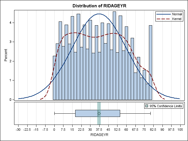
The diamond is the mean (37.19), and the line is the median (36.21).
* getting one graph at a time;
ods graphics on;
proc surveymeans data = nhanes2012 plots = boxplot;
weight wtint2yr;
cluster sdmvpsu;
strata sdmvstra;
var ridageyr;
run;
ods graphics off;
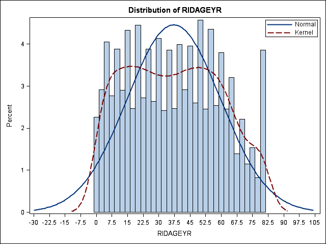
* getting just the histogram;
ods graphics on;
proc surveymeans data = nhanes2012 plots = histogram;
weight wtint2yr;
cluster sdmvpsu;
strata sdmvstra;
var ridageyr;
run;
ods graphics off;
There are a few different ways to get descriptive statistics with categorical
variables. You can use proc surveymeans if your variable is binary
(i.e., coded 0/1).
* descriptives with a binary variable;
* this is actually a proportion;
proc surveymeans data = nhanes2012;
weight wtint2yr;
cluster sdmvpsu;
strata sdmvstra;
var female;
run;
The SURVEYMEANS Procedure

            Data Summary

Number of Strata                  14
Number of Clusters                31
Number of Observations          9756
Sum of Weights             306590681


                                   Statistics

                                               Std Error
Variable               N            Mean         of Mean       95% CL for Mean
---------------------------------------------------------------------------------
female              9756        0.511952        0.006440    0.49836568 0.52553917
---------------------------------------------------------------------------------
Probably the most common procedure for getting descriptive statistics for
categorical variables is proc surveyfreq. The tables
statement in proc surveyfreq works the same way that the tables
statement in proc freq works.
* this might be more common;
proc surveyfreq data = nhanes2012;
weight wtint2yr;
cluster sdmvpsu;
strata sdmvstra;
tables female;
run;
The SURVEYFREQ Procedure

            Data Summary

Number of Strata                  14
Number of Clusters                31
Number of Observations          9756
Sum of Weights             306590681


                             Table of female

                          Weighted    Std Dev of               Std Err of
female     Frequency     Frequency      Wgt Freq    Percent       Percent
-------------------------------------------------------------------------
     0          4856     149630839       8783128    48.8048        0.6440
     1          4900     156959842      11234711    51.1952        0.6440

 Total          9756     306590681      19723273    100.000
-------------------------------------------------------------------------
You may want to use formats to help label the output.
* using formats;
proc surveyfreq data = nhanes2012;
weight wtint2yr;
cluster sdmvpsu;
strata sdmvstra;
tables female*dmdborn4;
format female fm. dmdborn4 cb.;
run;
The SURVEYFREQ Procedure

            Data Summary

Number of Strata                  14
Number of Clusters                31
Number of Observations          9756
Sum of Weights             306590681


                                Table of female by DMDBORN4

                                            Weighted    Std Dev of               Std Err of
female    DMDBORN4           Frequency     Frequency      Wgt Freq    Percent       Percent
-------------------------------------------------------------------------------------------
male      born elsewhere          1027      22449131       2368069     7.3247        0.8655
          born in US              3825     127102676       8587374    41.4710        0.6134

          Total                   4852     149551807       8773197    48.7957        0.6428
-------------------------------------------------------------------------------------------
female    born elsewhere          1056      23543299       1926175     7.6817        0.7451
          born in US              3843     133390830      11273589    43.5227        1.2458

          Total                   4899     156934129      11235137    51.2043        0.6428
-------------------------------------------------------------------------------------------
Total     born elsewhere          2083      45992430       4177655    15.0064        1.5756
          born in US              7668     260493506      19670647    84.9936        1.5756

          Total                   9751     306485936      19715992    100.000
-------------------------------------------------------------------------------------------
                                   Frequency Missing = 5
In the next example, several options were used. The expected option gives the expected frequencies for each cell in the
table. The row option gives the row percentages. The col option gives the column percentages. The
chisq option gives the Rao-Scott chi-square test; lrchisq option gives the likelihood ratio chi-square test; the wchisq
option gives the Wald chi-square test; the wllchisq option gives the Wald log-linear chi-square test.
proc surveyfreq data = nhanes2012;
weight wtint2yr;
cluster sdmvpsu;
strata sdmvstra;
tables female*dmdborn4 / expected row col chisq lrchisq wchisq wllchisq;
format female fm. dmdborn4 cb.;
run;
The SURVEYFREQ Procedure

            Data Summary

Number of Strata                  14
Number of Clusters                31
Number of Observations          9756
Sum of Weights             306590681


                                   Table of female by DMDBORN4

                                         Weighted   Std Dev of     Expected             Std Err of
female   DMDBORN4          Frequency    Frequency     Wgt Freq     Wgt Freq   Percent      Percent
--------------------------------------------------------------------------------------------------
male     born elsewhere         1027     22449131      2368069     22442305    7.3247       0.8655
         born in US             3825    127102676      8587374    127109501   41.4710       0.6134

         Total                  4852    149551807      8773197                48.7957       0.6428
--------------------------------------------------------------------------------------------------
female   born elsewhere         1056     23543299      1926175     23550124    7.6817       0.7451
         born in US             3843    133390830     11273589    133384005   43.5227       1.2458

         Total                  4899    156934129     11235137                51.2043       0.6428
--------------------------------------------------------------------------------------------------
Total    born elsewhere         2083     45992430      4177655                15.0064       1.5756
         born in US             7668    260493506     19670647                84.9936       1.5756

         Total                  9751    306485936     19715992                100.000
--------------------------------------------------------------------------------------------------
                                      Frequency Missing = 5

                       Table of female by DMDBORN4

                              Row     Std Err of     Column     Std Err of
female   DMDBORN4         Percent    Row Percent    Percent    Col Percent
--------------------------------------------------------------------------
male     born elsewhere   15.0109         1.6401    48.8105         1.2315
         born in US       84.9891         1.6401    48.7930         0.6756

         Total            100.000
--------------------------------------------------------------------------
female   born elsewhere   15.0020         1.5769    51.1895         1.2315
         born in US       84.9980         1.5769    51.2070         0.6756

         Total            100.000
--------------------------------------------------------------------------
Total    born elsewhere                             100.000
         born in US                                 100.000

         Total
--------------------------------------------------------------------------
                          Frequency Missing = 5
Table of female by DMDBORN4

 Rao-Scott Chi-Square Test

Pearson Chi-Square    0.0002
Design Correction     0.7893

Rao-Scott Chi-Square  0.0002
DF                         1
Pr > ChiSq            0.9889

F Value               0.0002
Num DF                     1
Den DF                    17
Pr > F                0.9891

     Sample Size = 9751


  Rao-Scott Likelihood Ratio Test

Likelihood Ratio Chi-Square  0.0002
Design Correction            0.7893

Rao-Scott Chi-Square         0.0002
DF                                1
Pr > ChiSq                   0.9889

F Value                      0.0002
Num DF                            1
Den DF                           17
Pr > F                       0.9891

        Sample Size = 9751


 Wald Chi-Square Test

Chi-Square      0.0002

F Value         0.0002
Num DF               1
Den DF              17
Pr > F          0.9891

  Sample Size = 9751
Table of female by DMDBORN4

Wald Log-Linear Chi-Square Test

Chi-Square      0.0002

F Value         0.0002
Num DF               1
Den DF              17
Pr > F          0.9891

  Sample Size = 9751
In the next example, we will use three options. The cv option displays coefficients of
variation for percentages. The definition of “coefficient of variation” is that it is the standard deviation / mean, or, in our case, the standard error
divided by the point estimate. For example, for males born elsewhere for the percentage, .8655/7.3247 =
.1182. The cvwt option displays coefficients of
variation for weighted frequencies. For example, for males born elsewhere:
2368069/22449131 = .1055. The deff option displays design effects for percentages. This attempts to quantify the extent to which
the observed sampling error differs from what would be expected if SRS had been used. It is defined as variance(observed) / variance(SRS). It can be thought of as a measure of efficiency. If the design effect is 1, then the current analysis
with the current sampling plan is as efficient as the same analysis using a SRS. If the design effect
is less than 1, then the current analysis with the current sample is more efficient than the same analysis
with SRS. If the design effect is greater than 1, then the current analysis with the current sample
is less efficient than the same analysis with a SRS. In general, clustering increases the design effect.
This is related to the idea of an “effective sample size”. For example, males born elsewhere: 1027/10.7602 = 95.44
total born elsewhere: 2083/18.9775 = 109.76.
proc surveyfreq data = nhanes2012;
weight wtint2yr;
cluster sdmvpsu;
strata sdmvstra;
tables female*dmdborn4 / cv cvwt deff;
format female fm. dmdborn4 cb.;
run;
The SURVEYFREQ Procedure

            Data Summary

Number of Strata                  14
Number of Clusters                31
Number of Observations          9756
Sum of Weights             306590681


                                   Table of female by DMDBORN4

                                         Weighted   Std Dev of      CV for             Std Err of
female   DMDBORN4          Frequency    Frequency     Wgt Freq    Wgt Freq   Percent      Percent
-------------------------------------------------------------------------------------------------
male     born elsewhere         1027     22449131      2368069      0.1055    7.3247       0.8655
         born in US             3825    127102676      8587374      0.0676   41.4710       0.6134

         Total                  4852    149551807      8773197      0.0587   48.7957       0.6428
-------------------------------------------------------------------------------------------------
female   born elsewhere         1056     23543299      1926175      0.0818    7.6817       0.7451
         born in US             3843    133390830     11273589      0.0845   43.5227       1.2458

         Total                  4899    156934129     11235137      0.0716   51.2043       0.6428
-------------------------------------------------------------------------------------------------
Total    born elsewhere         2083     45992430      4177655      0.0908   15.0064       1.5756
         born in US             7668    260493506     19670647      0.0755   84.9936       1.5756

         Total                  9751    306485936     19715992      0.0643   100.000
-------------------------------------------------------------------------------------------------
                                      Frequency Missing = 5

          Table of female by DMDBORN4

                             CV for      Design
female   DMDBORN4           Percent      Effect
-----------------------------------------------
male     born elsewhere      0.1182     10.7602
         born in US          0.0148      1.5114

         Total               0.0132      1.6126
-----------------------------------------------
female   born elsewhere      0.0970      7.6319
         born in US          0.0286      6.1566

         Total               0.0126      1.6126
-----------------------------------------------
Total    born elsewhere      0.1050     18.9775
         born in US          0.0185     18.9775

         Total
-----------------------------------------------
             Frequency Missing = 5
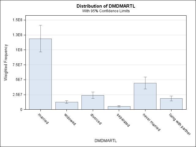
Let’s look at some graphs. Using the format will put the labels on the x-axis on the
graph.
ods graphics on;
proc surveyfreq data = nhanes2012;
weight wtint2yr;
cluster sdmvpsu;
strata sdmvstra;
tables dmdmartl / plots = wtfreqplot;
format dmdmartl matsat.;
run;
ods graphics off;

The SURVEYFREQ Procedure

            Data Summary

Number of Strata                  14
Number of Clusters                31
Number of Observations          9756
Sum of Weights             306590681


                                  Table of DMDMARTL

                                       Weighted    Std Dev of               Std Err of
DMDMARTL                Frequency     Frequency      Wgt Freq    Percent       Percent
--------------------------------------------------------------------------------------
married                      2683     118822198      10556102    53.0792        2.0495
widowed                       467      12586462       1087437     5.6225        0.3200
divorced                      571      23926362       2606988    10.6882        0.7248
separated                     204       5366932        614868     2.3975        0.3161
never married                1188      44479637       4687152    19.8695        2.3629
living with partner           440      18676762       1874572     8.3431        0.6473

Total                        5553     223858353      14237911    100.000
--------------------------------------------------------------------------------------
                               Frequency Missing = 4203
* choose more interesting variables;
ods graphics on;
proc surveyfreq data = nhanes2012;
weight wtint2yr;
cluster sdmvpsu;
strata sdmvstra;
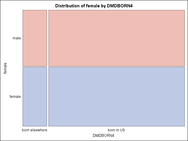
tables female*dmdborn4 / plots = mosaicplot;
format female fm. dmdborn4 cb.;
run;
ods graphics off;

The SURVEYFREQ Procedure

            Data Summary

Number of Strata                  14
Number of Clusters                31
Number of Observations          9756
Sum of Weights             306590681


                                Table of female by DMDBORN4

                                            Weighted    Std Dev of               Std Err of
female    DMDBORN4           Frequency     Frequency      Wgt Freq    Percent       Percent
-------------------------------------------------------------------------------------------
male      born elsewhere          1027      22449131       2368069     7.3247        0.8655
          born in US              3825     127102676       8587374    41.4710        0.6134

          Total                   4852     149551807       8773197    48.7957        0.6428
-------------------------------------------------------------------------------------------
female    born elsewhere          1056      23543299       1926175     7.6817        0.7451
          born in US              3843     133390830      11273589    43.5227        1.2458

          Total                   4899     156934129      11235137    51.2043        0.6428
-------------------------------------------------------------------------------------------
Total     born elsewhere          2083      45992430       4177655    15.0064        1.5756
          born in US              7668     260493506      19670647    84.9936        1.5756

          Total                   9751     306485936      19715992    100.000
-------------------------------------------------------------------------------------------
                                   Frequency Missing = 5
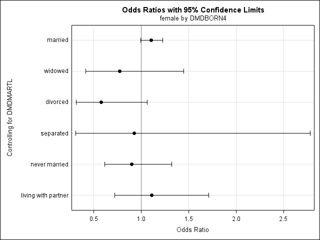
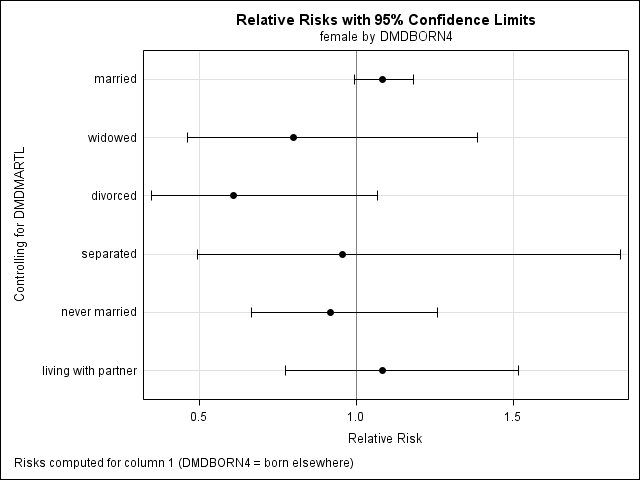
If you are requesting more than one plot, you need to enclose the plots in
parentheses. The or option will give the odds ratios, and the
risk option will give risks.
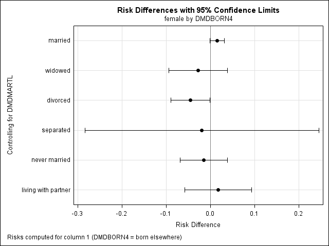
ods graphics on;
proc surveyfreq data = nhanes2012;
weight wtint2yr;
cluster sdmvpsu;
strata sdmvstra;
tables dmdmartl*female*dmdborn4 / risk or plots =(oddsratioplot relriskplot);
format dmdmartl matsat. female fm. dmdborn4 cb.;
run;
ods graphics off;
The SURVEYFREQ Procedure

            Data Summary

Number of Strata                  14
Number of Clusters                31
Number of Observations          9756
Sum of Weights             306590681


                                Table of female by DMDBORN4
                             Controlling for DMDMARTL=married

                                            Weighted    Std Dev of               Std Err of
female    DMDBORN4           Frequency     Frequency      Wgt Freq    Percent       Percent
-------------------------------------------------------------------------------------------
male      born elsewhere           554      11803069       1179456     9.9367        1.1615
          born in US               874      46849089       4983912    39.4410        1.0838

          Total                   1428      58652159       5189428    49.3777        0.5675
-------------------------------------------------------------------------------------------
female    born elsewhere           476      11167772       1125718     9.4019        1.0815
          born in US               777      48962647       5297262    41.2204        1.3449

          Total                   1253      60130420       5451479    50.6223        0.5675
-------------------------------------------------------------------------------------------
Total     born elsewhere          1030      22970842       2253478    19.3386        2.2056
          born in US              1651      95811737      10207366    80.6614        2.2056

          Total                   2681     118782579      10555944    100.000
-------------------------------------------------------------------------------------------


                Column 1 Risk Estimates

                        Standard
                Risk       Error   95% Confidence Limits

Row 1         0.2012      0.0228       0.1532     0.2492
Row 2         0.1857      0.0220       0.1393     0.2321
Total         0.1934      0.0221       0.1469     0.2399

Difference    0.0155      0.0078      -0.0010     0.0320

             Difference is (Row 1 - Row 2)

                   Sample Size = 5549
                Column 2 Risk Estimates

                        Standard
                Risk       Error   95% Confidence Limits

Row 1         0.7988      0.0228       0.7508     0.8468
Row 2         0.8143      0.0220       0.7679     0.8607
Total         0.8066      0.0221       0.7601     0.8531

Difference   -0.0155      0.0078      -0.0320     0.0010

             Difference is (Row 1 - Row 2)

                   Sample Size = 5549


           Odds Ratio and Relative Risks (Row1/Row2)

                            Estimate       95% Confidence Limits

Odds Ratio                    1.1046        0.9937        1.2278
Column 1 Relative Risk        1.0835        0.9944        1.1806
Column 2 Relative Risk        0.9809        0.9609        1.0014

                       Sample Size = 5549


                                Table of female by DMDBORN4
                             Controlling for DMDMARTL=widowed

                                            Weighted    Std Dev of               Std Err of
female    DMDBORN4           Frequency     Frequency      Wgt Freq    Percent       Percent
-------------------------------------------------------------------------------------------
male      born elsewhere            23        299145         63828     2.3767        0.5554
          born in US                99       2433302        326571    19.3327        2.1606

          Total                    122       2732447        337748    21.7094        2.3135
-------------------------------------------------------------------------------------------
female    born elsewhere            82       1350041        202386    10.7261        1.8146
          born in US               263       8503975        963871    67.5645        3.0838

          Total                    345       9854015        951308    78.2906        2.3135
-------------------------------------------------------------------------------------------
Total     born elsewhere           105       1649186        210849    13.1029        1.9883
          born in US               362      10937276       1100321    86.8971        1.9883

          Total                    467      12586462       1087437    100.000
-------------------------------------------------------------------------------------------
                Column 1 Risk Estimates

                        Standard
                Risk       Error   95% Confidence Limits

Row 1         0.1095      0.0237       0.0595     0.1594
Row 2         0.1370      0.0239       0.0865     0.1875
Total         0.1310      0.0199       0.0891     0.1730

Difference   -0.0275      0.0316      -0.0941     0.0391

             Difference is (Row 1 - Row 2)

                   Sample Size = 5549


                Column 2 Risk Estimates

                        Standard
                Risk       Error   95% Confidence Limits

Row 1         0.8905      0.0237       0.8406     0.9405
Row 2         0.8630      0.0239       0.8125     0.9135
Total         0.8690      0.0199       0.8270     0.9109

Difference    0.0275      0.0316      -0.0391     0.0941

             Difference is (Row 1 - Row 2)

                   Sample Size = 5549


           Odds Ratio and Relative Risks (Row1/Row2)

                            Estimate       95% Confidence Limits

Odds Ratio                    0.7744        0.4141        1.4482
Column 1 Relative Risk        0.7991        0.4607        1.3860
Column 2 Relative Risk        1.0319        0.9564        1.1134

                       Sample Size = 5549
                                Table of female by DMDBORN4
                             Controlling for DMDMARTL=divorced

                                            Weighted    Std Dev of               Std Err of
female    DMDBORN4           Frequency     Frequency      Wgt Freq    Percent       Percent
-------------------------------------------------------------------------------------------
male      born elsewhere            32        646692        190158     2.7028        0.8131
          born in US               205       8640920       1381509    36.1146        3.6127

          Total                    237       9287612       1406845    38.8175        3.6318
-------------------------------------------------------------------------------------------
female    born elsewhere            70       1676180        267604     7.0056        1.2917
          born in US               264      12962570       1692897    54.1769        3.5153

          Total                    334      14638749       1727388    61.1825        3.6318
-------------------------------------------------------------------------------------------
Total     born elsewhere           102       2322871        384346     9.7084        1.8069
          born in US               469      21603490       2586103    90.2916        1.8069

          Total                    571      23926362       2606988    100.000
-------------------------------------------------------------------------------------------


                Column 1 Risk Estimates

                        Standard
                Risk       Error   95% Confidence Limits

Row 1         0.0696      0.0211       0.0252     0.1141
Row 2         0.1145      0.0204       0.0715     0.1575
Total         0.0971      0.0181       0.0590     0.1352

Difference   -0.0449      0.0210      -0.0893    -0.0005

             Difference is (Row 1 - Row 2)

                   Sample Size = 5549


                Column 2 Risk Estimates

                        Standard
                Risk       Error   95% Confidence Limits

Row 1         0.9304      0.0211       0.8859     0.9748
Row 2         0.8855      0.0204       0.8425     0.9285
Total         0.9029      0.0181       0.8648     0.9410

             Difference is (Row 1 - Row 2)

                   Sample Size = 5549
                Column 2 Risk Estimates

                        Standard
                Risk       Error   95% Confidence Limits

Difference    0.0449      0.0210       0.0005     0.0893

             Difference is (Row 1 - Row 2)

                   Sample Size = 5549


           Odds Ratio and Relative Risks (Row1/Row2)

                            Estimate       95% Confidence Limits

Odds Ratio                    0.5788        0.3154        1.0619
Column 1 Relative Risk        0.6081        0.3466        1.0669
Column 2 Relative Risk        1.0507        1.0006        1.1033

                       Sample Size = 5549


                                Table of female by DMDBORN4
                            Controlling for DMDMARTL=separated

                                            Weighted    Std Dev of               Std Err of
female    DMDBORN4           Frequency     Frequency      Wgt Freq    Percent       Percent
-------------------------------------------------------------------------------------------
male      born elsewhere            36        798720        216266    14.8822        3.5300
          born in US                43       1220641        289387    22.7437        4.3090

          Total                     79       2019361        376397    37.6260        4.7175
-------------------------------------------------------------------------------------------
female    born elsewhere            54       1387134        213988    25.8459        3.9489
          born in US                71       1960437        364269    36.5281        4.9696

          Total                    125       3347571        413911    62.3740        4.7175
-------------------------------------------------------------------------------------------
Total     born elsewhere            90       2185854        249474    40.7282        3.2853
          born in US               114       3181078        458084    59.2718        3.2853

          Total                    204       5366932        614868    100.000
-------------------------------------------------------------------------------------------
                Column 1 Risk Estimates

                        Standard
                Risk       Error   95% Confidence Limits

Row 1         0.3955      0.0822       0.2222     0.5689
Row 2         0.4144      0.0599       0.2880     0.5408
Total         0.4073      0.0329       0.3380     0.4766

Difference   -0.0188      0.1254      -0.2835     0.2458

             Difference is (Row 1 - Row 2)

                   Sample Size = 5549


                Column 2 Risk Estimates

                        Standard
                Risk       Error   95% Confidence Limits

Row 1         0.6045      0.0822       0.4311     0.7778
Row 2         0.5856      0.0599       0.4592     0.7120
Total         0.5927      0.0329       0.5234     0.6620

Difference    0.0188      0.1254      -0.2458     0.2835

             Difference is (Row 1 - Row 2)

                   Sample Size = 5549


           Odds Ratio and Relative Risks (Row1/Row2)

                            Estimate       95% Confidence Limits

Odds Ratio                    0.9248        0.3077        2.7793
Column 1 Relative Risk        0.9545        0.4948        1.8413
Column 2 Relative Risk        1.0322        0.6625        1.6082

                       Sample Size = 5549
                                Table of female by DMDBORN4
                          Controlling for DMDMARTL=never married

                                            Weighted    Std Dev of               Std Err of
female    DMDBORN4           Frequency     Frequency      Wgt Freq    Percent       Percent
-------------------------------------------------------------------------------------------
male      born elsewhere           150       3945129        570145     8.8807        1.1797
          born in US               482      21151252       2485409    47.6125        1.9035

          Total                    632      25096380       2750788    56.4931        1.9690
-------------------------------------------------------------------------------------------
female    born elsewhere           133       3316186        623580     7.4649        1.1880
          born in US               421      16011195       2027247    36.0420        2.3406

          Total                    554      19327382       2250319    43.5069        1.9690
-------------------------------------------------------------------------------------------
Total     born elsewhere           283       7261315       1072947    16.3456        2.0345
          born in US               903      37162447       4176512    83.6544        2.0345

          Total                   1186      44423762       4681954    100.000
-------------------------------------------------------------------------------------------


                Column 1 Risk Estimates

                        Standard
                Risk       Error   95% Confidence Limits

Row 1         0.1572      0.0196       0.1158     0.1986
Row 2         0.1716      0.0287       0.1110     0.2321
Total         0.1635      0.0203       0.1205     0.2064

Difference   -0.0144      0.0254      -0.0680     0.0393

             Difference is (Row 1 - Row 2)

                   Sample Size = 5549


                Column 2 Risk Estimates

                        Standard
                Risk       Error   95% Confidence Limits

Row 1         0.8428      0.0196       0.8014     0.8842
Row 2         0.8284      0.0287       0.7679     0.8890
Total         0.8365      0.0203       0.7936     0.8795

             Difference is (Row 1 - Row 2)

                   Sample Size = 5549
                Column 2 Risk Estimates

                        Standard
                Risk       Error   95% Confidence Limits

Difference    0.0144      0.0254      -0.0393     0.0680

             Difference is (Row 1 - Row 2)

                   Sample Size = 5549


           Odds Ratio and Relative Risks (Row1/Row2)

                            Estimate       95% Confidence Limits

Odds Ratio                    0.9006        0.6143        1.3202
Column 1 Relative Risk        0.9162        0.6665        1.2593
Column 2 Relative Risk        1.0174        0.9537        1.0853

                       Sample Size = 5549


                                Table of female by DMDBORN4
                       Controlling for DMDMARTL=living with partner

                                            Weighted    Std Dev of               Std Err of
female    DMDBORN4           Frequency     Frequency      Wgt Freq    Percent       Percent
-------------------------------------------------------------------------------------------
male      born elsewhere            69       2257394        449540    12.0866        1.9362
          born in US               168       7272128        876424    38.9368        2.4468

          Total                    237       9529522       1065259    51.0234        1.7000
-------------------------------------------------------------------------------------------
female    born elsewhere            64       2000636        413700    10.7119        2.0043
          born in US               139       7146604        832299    38.2647        2.5917

          Total                    203       9147240        910699    48.9766        1.7000
-------------------------------------------------------------------------------------------
Total     born elsewhere           133       4258030        799318    22.7985        3.5450
          born in US               307      14418732       1572309    77.2015        3.5450

          Total                    440      18676762       1874572    100.000
-------------------------------------------------------------------------------------------
                Column 1 Risk Estimates

                        Standard
                Risk       Error   95% Confidence Limits

Row 1         0.2369      0.0380       0.1567     0.3170
Row 2         0.2187      0.0414       0.1313     0.3061
Total         0.2280      0.0355       0.1532     0.3028

Difference    0.0182      0.0358      -0.0574     0.0937

             Difference is (Row 1 - Row 2)

                   Sample Size = 5549


                Column 2 Risk Estimates

                        Standard
                Risk       Error   95% Confidence Limits

Row 1         0.7631      0.0380       0.6830     0.8433
Row 2         0.7813      0.0414       0.6939     0.8687
Total         0.7720      0.0355       0.6972     0.8468

Difference   -0.0182      0.0358      -0.0937     0.0574

             Difference is (Row 1 - Row 2)

                   Sample Size = 5549


           Odds Ratio and Relative Risks (Row1/Row2)

                            Estimate       95% Confidence Limits

Odds Ratio                    1.1089        0.7191        1.7100
Column 1 Relative Risk        1.0831        0.7741        1.5155
Column 2 Relative Risk        0.9767        0.8859        1.0769

                       Sample Size = 5549
Analysis of subpopulations
Before we continue, we should pause to discuss the analysis of
subpopulations. The analysis of subpopulations is one place where survey
data and experimental data are quite different. If you have data from an
experiment (or quasi-experiment), and you want to analyze the responses from,
say, just the women, or just people over age 50, you can just delete the
unwanted cases from the data set or use a by statement.
Survey data are different. With survey data, you (almost) never get to delete
any cases from the data set, even if you will never use them in any of your
analyses. Because of the way the by statement works, you usually don’t use
it with survey data either. Instead, SAS has provided a domain
statement in most survey procedures that allows you to correctly analyze
subpopulations of your survey data. A domain and a subpopulation are the
same thing. The domain statement is very similar to using a by
statement in that you will get output for each level of the variable (or
variables) listed on the statement. This means that you will often times
get more output that you want; you simply ignore the output for domains that are
not of interest to you. Please note that there is no domain
statement in proc surveyfreq; you are expected to include the variables
that you would have put on the domain statement on the tables statement.
First, however, let’s take a second to see why deleting cases from a survey
data set can be so problematic. If the data set is subset (meaning that
observations not to be included in the subpopulation are deleted from the data
set), two problems arise. First, the estimated number of elements in the population
cannot be correctly calculated because some numbers are missing as you sum down
the column of sampling weights. Secondly, the standard errors of the estimates
cannot be calculated correctly. When
the subpopulation option(s) is used, only the cases defined by the subpopulation
are used in the calculation of the estimate, but all cases are used in the
calculation of the standard errors. For more information on this issue, please
see
Sampling Techniques, Third Edition by William G. Cochran (1977) and
Small Area Estimation by J. N. K. Rao (2003).
We will begin with an analysis that we have seen before.
* subpops;
proc surveymeans data = nhanes2012;
weight wtint2yr;
cluster sdmvpsu;
strata sdmvstra;
var pad630;
run;
The SURVEYMEANS Procedure

            Data Summary

Number of Strata                  14
Number of Clusters                31
Number of Observations          9756
Sum of Weights             306590681


                                   Statistics

                                               Std Error
Variable               N            Mean         of Mean       95% CL for Mean
---------------------------------------------------------------------------------
PAD630              2054      139.887377        5.579060    128.116590 151.658164
---------------------------------------------------------------------------------
Now let’s add the domain statement. The format statement
is not technically needed, but it is a nice way to more clearly label the
output. If you were interested only in the mean for females, you would
ignore the output for males.
proc surveymeans data = nhanes2012;
weight wtint2yr;
cluster sdmvpsu;
strata sdmvstra;
domain female;
var pad630;
format female fm.;
run;
The SURVEYMEANS Procedure

            Data Summary

Number of Strata                  14
Number of Clusters                31
Number of Observations          9756
Sum of Weights             306590681


                                   Statistics

                                               Std Error
Variable               N            Mean         of Mean       95% CL for Mean
---------------------------------------------------------------------------------
PAD630              2054      139.887377        5.579060    128.116590 151.658164
---------------------------------------------------------------------------------


                                  Domain Analysis: female

                                                         Std Error
female    Variable               N            Mean         of Mean       95% CL for Mean
-------------------------------------------------------------------------------------------
male      PAD630              1136      155.627196        7.008380    140.840807 170.413584
female    PAD630               918      121.684284        5.352345    110.391824 132.976744
-------------------------------------------------------------------------------------------
In this example, we include two variables on the domain statement.
Notice that this is the same as running proc surveymeans twice with each
of the variables on the domain statement in turn.
proc surveymeans data = nhanes2012;
weight wtint2yr;
cluster sdmvpsu;
strata sdmvstra;
domain female dmdmartl;
var pad630;
format dmdmartl matsat. female fm.;
run;
The SURVEYMEANS Procedure

            Data Summary

Number of Strata                  14
Number of Clusters                31
Number of Observations          9756
Sum of Weights             306590681


                                   Statistics

                                               Std Error
Variable               N            Mean         of Mean       95% CL for Mean
---------------------------------------------------------------------------------
PAD630              2054      139.887377        5.579060    128.116590 151.658164
---------------------------------------------------------------------------------


                                  Domain Analysis: female

                                                         Std Error
female    Variable               N            Mean         of Mean       95% CL for Mean
-------------------------------------------------------------------------------------------
male      PAD630              1136      155.627196        7.008380    140.840807 170.413584
female    PAD630               918      121.684284        5.352345    110.391824 132.976744
-------------------------------------------------------------------------------------------


                                  Domain Analysis: DMDMARTL

                                                              Std Error
DMDMARTL             Variable             N          Mean       of Mean     95% CL for Mean
----------------------------------------------------------------------------------------------
married              PAD630             841    139.439779      6.869524  124.946351 153.933208
widowed              PAD630              96    122.878708      9.530837  102.770399 142.987017
divorced             PAD630             166    164.023980     12.070142  138.558206 189.489754
separated            PAD630              70    195.067692     37.432563  116.091889 274.043496
never married        PAD630             363    140.786819     10.691710  118.229282 163.344355
living with partner  PAD630             169    165.483679     10.304480  143.743126 187.224232
----------------------------------------------------------------------------------------------
In this example, we cross the domain variables, giving us each combination of
the two variables.
proc surveymeans data = nhanes2012;
weight wtint2yr;
cluster sdmvpsu;
strata sdmvstra;
domain female*dmdmartl;
var pad630;
format dmdmartl matsat. female fm.;
run;
The SURVEYMEANS Procedure

            Data Summary

Number of Strata                  14
Number of Clusters                31
Number of Observations          9756
Sum of Weights             306590681


                                   Statistics

                                               Std Error
Variable               N            Mean         of Mean       95% CL for Mean
---------------------------------------------------------------------------------
PAD630              2054      139.887377        5.579060    128.116590 151.658164
---------------------------------------------------------------------------------


                            Domain Analysis: female*DMDMARTL

                                                                                Std Error
female    DMDMARTL               Variable               N            Mean         of Mean
-----------------------------------------------------------------------------------------
male      married                PAD630               494      156.694056        8.765612
          widowed                PAD630                23      132.611146       20.775755
          divorced               PAD630                77      209.422973       27.286194
          separated              PAD630                32      187.968526       38.861059
          never married          PAD630               214      146.423066       12.353287
          living with partner    PAD630               102      201.422030       13.418949
female    married                PAD630               347      118.625504        9.590405
          widowed                PAD630                73      120.956913       11.104393
          divorced               PAD630                89      124.634331       15.505908
          separated              PAD630                38      200.933304       52.499861
-----------------------------------------------------------------------------------------


                 Domain Analysis: female*DMDMARTL

female    DMDMARTL               Variable       95% CL for Mean
------------------------------------------------------------------
male      married                PAD630      138.200232 175.187881
          widowed                PAD630       88.778134 176.444159
          divorced               PAD630      151.854136 266.991811
          separated              PAD630      105.978858 269.958193
          never married          PAD630      120.359908 172.486223
          living with partner    PAD630      173.110522 229.733538
female    married                PAD630       98.391518 138.859490
          widowed                PAD630       97.528692 144.385134
          divorced               PAD630       91.919726 157.348937
          separated              PAD630       90.168280 311.698328
------------------------------------------------------------------
                            Domain Analysis: female*DMDMARTL

                                                                                Std Error
female    DMDMARTL               Variable               N            Mean         of Mean
-----------------------------------------------------------------------------------------
female    never married          PAD630               149      131.709083       13.305583
          living with partner    PAD630                67      122.573635       14.885114
-----------------------------------------------------------------------------------------


                 Domain Analysis: female*DMDMARTL

female    DMDMARTL               Variable       95% CL for Mean
------------------------------------------------------------------
female    never married          PAD630      103.636758 159.781409
          living with partner    PAD630       91.168789 153.978481
------------------------------------------------------------------
In this example, we cross three variables on the domain statement.
proc surveymeans data = nhanes2012;
weight wtint2yr;
cluster sdmvpsu;
strata sdmvstra;
domain female*dmdmartl*dmdeduc2;
var pad630;
format dmdmartl matsat. female fm. dmdeduc2 edu.;
run;
The SURVEYMEANS Procedure

            Data Summary

Number of Strata                  14
Number of Clusters                31
Number of Observations          9756
Sum of Weights             306590681


                                   Statistics

                                               Std Error
Variable               N            Mean         of Mean       95% CL for Mean
---------------------------------------------------------------------------------
PAD630              2054      139.887377        5.579060    128.116590 151.658164
---------------------------------------------------------------------------------


                            Domain Analysis: female*DMDMARTL*DMDEDUC2

female   DMDMARTL              DMDEDUC2                    Variable              N           Mean
-------------------------------------------------------------------------------------------------
male     married               less than 9th grade         PAD630               44     175.262504
                               no hs diploma               PAD630               68     191.892326
                               hs grad or GED              PAD630              111     165.884895
                               some college or AA degree   PAD630              166     155.183990
-------------------------------------------------------------------------------------------------

                    Domain Analysis: female*DMDMARTL*DMDEDUC2

                                                                         Std Error
female   DMDMARTL              DMDEDUC2                    Variable        of Mean
----------------------------------------------------------------------------------
male     married               less than 9th grade         PAD630        28.123585
                               no hs diploma               PAD630        18.189105
                               hs grad or GED              PAD630         9.758340
                               some college or AA degree   PAD630        13.216380
----------------------------------------------------------------------------------


                         Domain Analysis: female*DMDMARTL*DMDEDUC2

female   DMDMARTL              DMDEDUC2                    Variable      95% CL for Mean
-------------------------------------------------------------------------------------------
male     married               less than 9th grade         PAD630     115.926926 234.598081
                               no hs diploma               PAD630     153.516670 230.267982
                               hs grad or GED              PAD630     145.296598 186.473193
                               some college or AA degree   PAD630     127.299865 183.068115
-------------------------------------------------------------------------------------------
The SURVEYMEANS Procedure


                            Domain Analysis: female*DMDMARTL*DMDEDUC2

female   DMDMARTL              DMDEDUC2                    Variable              N           Mean
-------------------------------------------------------------------------------------------------
male     married               college grad or above       PAD630              105     133.266995
         widowed               less than 9th grade         PAD630                4     187.343598
                               no hs diploma               PAD630                4     167.204010
                               hs grad or GED              PAD630                2     103.256927
                               some college or AA degree   PAD630                9     125.939470
                               college grad or above       PAD630                4     123.887738
         divorced              less than 9th grade         PAD630                0              .
                               no hs diploma               PAD630               13     238.105548
                               hs grad or GED              PAD630               28     159.620092
                               some college or AA degree   PAD630               28     271.147197
                               college grad or above       PAD630                8     181.383414
         separated             less than 9th grade         PAD630                6     205.133253
                               no hs diploma               PAD630                7     199.085099
                               hs grad or GED              PAD630                9     279.838117
                               some college or AA degree   PAD630                8      81.121846
                               college grad or above       PAD630                2     237.326057
         never married         less than 9th grade         PAD630                8     221.332123
                               no hs diploma               PAD630               24     260.453605
                               hs grad or GED              PAD630               53     169.780030
                               some college or AA degree   PAD630               93     125.941216
                               college grad or above       PAD630               36     104.576598
         living with partner   less than 9th grade         PAD630                9     188.915139
                               no hs diploma               PAD630               21     257.398122
                               hs grad or GED              PAD630               28     215.157719
                               some college or AA degree   PAD630               36     198.181294
                               college grad or above       PAD630                8     105.547477
female   married               less than 9th grade         PAD630               14     123.187262
                               no hs diploma               PAD630               36     143.361616
                               hs grad or GED              PAD630               60     111.808026
                               some college or AA degree   PAD630              121     146.288791
                               college grad or above       PAD630              116      88.919333
         widowed               less than 9th grade         PAD630                5     176.095932
                               no hs diploma               PAD630               17      90.605348
                               hs grad or GED              PAD630               15     110.480512
                               some college or AA degree   PAD630               27     101.838525
                               college grad or above       PAD630                9     260.996206
         divorced              less than 9th grade         PAD630                3      54.288869
                               no hs diploma               PAD630               10     163.202217
                               hs grad or GED              PAD630               23     145.507378
                               some college or AA degree   PAD630               39     129.588332
                               college grad or above       PAD630               14      76.006626
         separated             less than 9th grade         PAD630                4     169.359877
                               no hs diploma               PAD630               10     165.848237
                               hs grad or GED              PAD630               10     302.022494
                               some college or AA degree   PAD630               10     142.532187
-------------------------------------------------------------------------------------------------
The SURVEYMEANS Procedure

                    Domain Analysis: female*DMDMARTL*DMDEDUC2

                                                                         Std Error
female   DMDMARTL              DMDEDUC2                    Variable        of Mean
----------------------------------------------------------------------------------
male     married               college grad or above       PAD630        10.848793
         widowed               less than 9th grade         PAD630        62.966878
                               no hs diploma               PAD630        14.100541
                               hs grad or GED              PAD630        20.074215
                               some college or AA degree   PAD630        35.754504
                               college grad or above       PAD630        52.934045
         divorced              less than 9th grade         PAD630                .
                               no hs diploma               PAD630        29.710731
                               hs grad or GED              PAD630        17.529990
                               some college or AA degree   PAD630        56.919768
                               college grad or above       PAD630        33.002598
         separated             less than 9th grade         PAD630        35.534816
                               no hs diploma               PAD630        38.033471
                               hs grad or GED              PAD630        48.201023
                               some college or AA degree   PAD630        29.502335
                               college grad or above       PAD630        84.810682
         never married         less than 9th grade         PAD630        60.764206
                               no hs diploma               PAD630        41.069041
                               hs grad or GED              PAD630        18.531657
                               some college or AA degree   PAD630        11.381655
                               college grad or above       PAD630        26.159027
         living with partner   less than 9th grade         PAD630        71.240615
                               no hs diploma               PAD630        43.612166
                               hs grad or GED              PAD630        24.033974
                               some college or AA degree   PAD630        25.916937
                               college grad or above       PAD630         7.580480
female   married               less than 9th grade         PAD630        33.994125
                               no hs diploma               PAD630        14.005356
                               hs grad or GED              PAD630        12.927725
                               some college or AA degree   PAD630        22.892464
                               college grad or above       PAD630         8.306940
         widowed               less than 9th grade         PAD630        72.509645
                               no hs diploma               PAD630        17.212933
                               hs grad or GED              PAD630        37.211889
                               some college or AA degree   PAD630        11.742558
                               college grad or above       PAD630        63.187041
         divorced              less than 9th grade         PAD630        15.497090
                               no hs diploma               PAD630        47.287308
                               hs grad or GED              PAD630        25.434714
                               some college or AA degree   PAD630        28.490532
                               college grad or above       PAD630        11.322661
         separated             less than 9th grade         PAD630        80.576093
                               no hs diploma               PAD630        46.573934
                               hs grad or GED              PAD630       117.298227
                               some college or AA degree   PAD630        26.011047
----------------------------------------------------------------------------------
The SURVEYMEANS Procedure


                         Domain Analysis: female*DMDMARTL*DMDEDUC2

female   DMDMARTL              DMDEDUC2                    Variable      95% CL for Mean
-------------------------------------------------------------------------------------------
male     married               college grad or above       PAD630     110.378042 156.155948
         widowed               less than 9th grade         PAD630      54.495098 320.192099
                               no hs diploma               PAD630     137.454469 196.953551
                               hs grad or GED              PAD630      60.904035 145.609819
                               some college or AA degree   PAD630      50.504061 201.374879
                               college grad or above       PAD630      12.206665 235.568810
         divorced              less than 9th grade         PAD630              .          .
                               no hs diploma               PAD630     175.421385 300.789710
                               hs grad or GED              PAD630     122.635045 196.605139
                               some college or AA degree   PAD630     151.056984 391.237409
                               college grad or above       PAD630     111.754017 251.012810
         separated             less than 9th grade         PAD630     130.161344 280.105162
                               no hs diploma               PAD630     118.841490 279.328709
                               hs grad or GED              PAD630     178.142847 381.533387
                               some college or AA degree   PAD630      18.877360 143.366332
                               college grad or above       PAD630      58.391158 416.260955
         never married         less than 9th grade         PAD630      93.130856 349.533391
                               no hs diploma               PAD630     173.805502 347.101708
                               hs grad or GED              PAD630     130.681652 208.878407
                               some college or AA degree   PAD630     101.928024 149.954409
                               college grad or above       PAD630      49.385875 159.767320
         living with partner   less than 9th grade         PAD630      38.610579 339.219699
                               no hs diploma               PAD630     165.384495 349.411749
                               hs grad or GED              PAD630     164.450467 265.864972
                               some college or AA degree   PAD630     143.501336 252.861252
                               college grad or above       PAD630      89.554062 121.540892
female   married               less than 9th grade         PAD630      51.465926 194.908597
                               no hs diploma               PAD630     113.812897 172.910335
                               hs grad or GED              PAD630      84.532910 139.083141
                               some college or AA degree   PAD630      97.989913 194.587668
                               college grad or above       PAD630      71.393222 106.445445
         widowed               less than 9th grade         PAD630      23.113955 329.077910
                               no hs diploma               PAD630      54.289234 126.921462
                               hs grad or GED              PAD630      31.970289 188.990735
                               some college or AA degree   PAD630      77.063892 126.613157
                               college grad or above       PAD630     127.683203 394.309208
         divorced              less than 9th grade         PAD630      21.592867  86.984872
                               no hs diploma               PAD630      63.434717 262.969717
                               hs grad or GED              PAD630      91.844821 199.169934
                               some college or AA degree   PAD630      69.478564 189.698101
                               college grad or above       PAD630      52.117900  99.895353
         separated             less than 9th grade         PAD630      -0.640820 339.360573
                               no hs diploma               PAD630      67.585825 264.110649
                               hs grad or GED              PAD630      54.544868 549.500120
                               some college or AA degree   PAD630      87.653676 197.410699
-------------------------------------------------------------------------------------------
The SURVEYMEANS Procedure


                            Domain Analysis: female*DMDMARTL*DMDEDUC2

female   DMDMARTL              DMDEDUC2                    Variable              N           Mean
-------------------------------------------------------------------------------------------------
female   separated             college grad or above       PAD630                4     117.921631
         never married         less than 9th grade         PAD630                4     309.991244
                               no hs diploma               PAD630               10     166.333455
                               hs grad or GED              PAD630               19     190.285276
                               some college or AA degree   PAD630               79     109.549232
                               college grad or above       PAD630               37     126.519184
         living with partner   less than 9th grade         PAD630                2     120.000000
                               no hs diploma               PAD630                9     144.995045
                               hs grad or GED              PAD630               17      98.815434
                               some college or AA degree   PAD630               26     152.592251
                               college grad or above       PAD630               13      89.011298
-------------------------------------------------------------------------------------------------

                    Domain Analysis: female*DMDMARTL*DMDEDUC2

                                                                         Std Error
female   DMDMARTL              DMDEDUC2                    Variable        of Mean
----------------------------------------------------------------------------------
female   separated             college grad or above       PAD630        34.795950
         never married         less than 9th grade         PAD630        93.152302
                               no hs diploma               PAD630        46.458980
                               hs grad or GED              PAD630        55.647515
                               some college or AA degree   PAD630        15.629741
                               college grad or above       PAD630        19.292689
         living with partner   less than 9th grade         PAD630                0
                               no hs diploma               PAD630        24.397178
                               hs grad or GED              PAD630        21.160766
                               some college or AA degree   PAD630        23.746801
                               college grad or above       PAD630        23.175916
----------------------------------------------------------------------------------


                         Domain Analysis: female*DMDMARTL*DMDEDUC2

female   DMDMARTL              DMDEDUC2                    Variable      95% CL for Mean
-------------------------------------------------------------------------------------------
female   separated             college grad or above       PAD630      44.508594 191.334667
         never married         less than 9th grade         PAD630     113.457066 506.525422
                               no hs diploma               PAD630      68.313575 264.353336
                               hs grad or GED              PAD630      72.879282 307.691269
                               some college or AA degree   PAD630      76.573361 142.525104
                               college grad or above       PAD630      85.815170 167.223199
         living with partner   less than 9th grade         PAD630     120.000000 120.000000
                               no hs diploma               PAD630      93.521499 196.468590
                               hs grad or GED              PAD630      54.170121 143.460748
-------------------------------------------------------------------------------------------
The SURVEYMEANS Procedure


                         Domain Analysis: female*DMDMARTL*DMDEDUC2

female   DMDMARTL              DMDEDUC2                    Variable      95% CL for Mean
-------------------------------------------------------------------------------------------
female   living with partner   some college or AA degree   PAD630     102.490879 202.693622
                               college grad or above       PAD630      40.114391 137.908206
-------------------------------------------------------------------------------------------
By using proc print, we can see that there are only two cases that
have a valid value for pad630 in subpopulation females who are living
with a partner and have less than nine years of education, and both of those
values are 120. This is why no standard error can be estimated.
proc print data = nhanes2012;
var pad630;
where female = 1 and dmdmartl = 6 and dmdeduc2 = 1;
run;
 Obs    PAD630

 344      120
 479        .
1339        .
1962        .
1987      120
2075        .
2148        .
2178        .
2631        .
2972        .
3148        .
4118        .
4595        .
6610        .
7064        .
7112        .
7214        .
7709        .
7829        .
8095        .
8479        .
Now let’s say that you want to compare the means from two domains. In
this example, we get the mean of pad630 for females and males.
proc surveymeans data = nhanes2012;
weight wtint2yr;
cluster sdmvpsu;
strata sdmvstra;
domain female;
var pad630;
format female fm.;
run;
The SURVEYMEANS Procedure

            Data Summary

Number of Strata                  14
Number of Clusters                31
Number of Observations          9756
Sum of Weights             306590681


                                   Statistics

                                               Std Error
Variable               N            Mean         of Mean       95% CL for Mean
---------------------------------------------------------------------------------
PAD630              2054      139.887377        5.579060    128.116590 151.658164
---------------------------------------------------------------------------------


                                  Domain Analysis: female

                                                         Std Error
female    Variable               N            Mean         of Mean       95% CL for Mean
-------------------------------------------------------------------------------------------
male      PAD630              1136      155.627196        7.008380    140.840807 170.413584
female    PAD630               918      121.684284        5.352345    110.391824 132.976744
-------------------------------------------------------------------------------------------
There are a few different ways that you could compare 155.63 and 121.68.
In this example, we will use proc surveyreg and the contrast
statement. Notice that the output in the section titled Estimated
Regression Coefficients is almost identical to the output of the proc
surveymeans above.
proc surveyreg data = nhanes2012;
weight wtint2yr;
cluster sdmvpsu;
strata sdmvstra;
class female;
model pad630 = female / noint solution vadjust = none;
contrast 'comparing males and females' female 1 -1;
format female fm.;
run;
The SURVEYREG Procedure

Regression Analysis for Dependent Variable PAD630

            Data Summary

Number of Observations           2054
Sum of Weights               88768571
Weighted Mean of PAD630     139.88738
Weighted Sum of PAD630     1.24176E10


         Design Summary

Number of Strata              14
Number of Clusters            31


      Fit Statistics

R-square            0.5545
Root MSE            126.37
Denominator DF          17


       Class Level Information

CLASS
Variable      Levels    Values

female             2    female male


       Tests of Model Effects

Effect    Num DF    F Value    Pr > F

Model          2     325.56    <.0001
female         2     325.56    <.0001

NOTE: The denominator degrees of freedom for the F tests is 17.


               Estimated Regression Coefficients

                                 Standard
Parameter          Estimate         Error    t Value    Pr > |t|

female female    121.684284    5.35234462      22.73      <.0001
female male      155.627196    7.00837974      22.21      <.0001

NOTE: The denominator degrees of freedom for the t tests is 17.
Regression Analysis for Dependent Variable PAD630

                  Analysis of Contrasts

Contrast                       Num DF    F Value    Pr > F

comparing males and females         1      31.67    <.0001

NOTE: The denominator degrees of freedom for the F tests is 17.
In this example, we do the same analysis using proc surveymeans and
the lsmeans statement. This example is adapted from code on the SAS
website here.
proc surveyreg data = nhanes2012;
weight wtint2yr;
cluster sdmvpsu;
strata sdmvstra;
class female;
model pad630 = female / noint solution vadjust = none;
lsmeans female / diff;
format female fm.;
run;
The SURVEYREG Procedure

Regression Analysis for Dependent Variable PAD630

            Data Summary

Number of Observations           2054
Sum of Weights               88768571
Weighted Mean of PAD630     139.88738
Weighted Sum of PAD630     1.24176E10


         Design Summary

Number of Strata              14
Number of Clusters            31


      Fit Statistics

R-square            0.5545
Root MSE            126.37
Denominator DF          17


       Class Level Information

CLASS
Variable      Levels    Values

female             2    female male


       Tests of Model Effects

Effect    Num DF    F Value    Pr > F

Model          2     325.56    <.0001
female         2     325.56    <.0001

NOTE: The denominator degrees of freedom for the F tests is 17.


               Estimated Regression Coefficients

                                 Standard
Parameter          Estimate         Error    t Value    Pr > |t|

female female    121.684284    5.35234462      22.73      <.0001
female male      155.627196    7.00837974      22.21      <.0001

NOTE: The denominator degrees of freedom for the t tests is 17.
Regression Analysis for Dependent Variable PAD630

                  female Least Squares Means

                      Standard
female    Estimate       Error       DF    t Value    Pr > |t|

female      121.68      5.3523       17      22.73      <.0001
male        155.63      7.0084       17      22.21      <.0001


                Differences of female Least Squares Means

                                 Standard
female    _female    Estimate       Error       DF    t Value    Pr > |t|

female    male       -33.9429      6.0314       17      -5.63      <.0001
If you square the t-value from this analysis, you will get the F-value given
in the previous proc surveyreg analysis. The estimate of -33.94 is
simply the difference of the means, 121.68 – 155.63 (with a little rounding
error).
Regression
Now we will look at a few examples of regression analyses. We will use
proc surveyreg and proc surveylogistic. The variables in
these examples were chosen because they were either continuous or categorical,
not because of data that they contain. In other words, the models shown
here were not constructed to make substantive sense; rather, they were
constructed to illustrate how certain things can be done. The variable pad630 is the
number of minutes spent doing moderate-intensity activities on a typical work day.
proc surveyreg data = nhanes2012;
weight wtint2yr;
cluster sdmvpsu;
strata sdmvstra;
class female;
model pad630 = female ridageyr / solution;
format female fm.;
run;
The SURVEYREG Procedure

Regression Analysis for Dependent Variable PAD630

            Data Summary

Number of Observations           2054
Sum of Weights               88768571
Weighted Mean of PAD630     139.88738
Weighted Sum of PAD630     1.24176E10


         Design Summary

Number of Strata              14
Number of Clusters            31


      Fit Statistics

R-Square           0.01933
Root MSE            126.29
Denominator DF          17


       Class Level Information

CLASS
Variable      Levels    Values

female             2    female male


         Tests of Model Effects

Effect       Num DF    F Value    Pr > F

Model             2      18.23    <.0001
Intercept         1     327.92    <.0001
female            1      30.26    <.0001
RIDAGEYR          1       4.97    0.0396

NOTE: The denominator degrees of freedom for the F tests is 17.


               Estimated Regression Coefficients

                                 Standard
Parameter          Estimate         Error    t Value    Pr > |t|

Intercept        167.289537    9.31899525      17.95      <.0001
female female    -33.125134    6.02167950      -5.50      <.0001
female male        0.000000    0.00000000        .         .
RIDAGEYR          -0.287604    0.12906252      -2.23      0.0396

NOTE: The degrees of freedom for the t tests is 17.
      Matrix X'WX is singular and a generalized inverse was used to solve the normal equations.
      Estimates are not unique.
There is a class
statement in proc surveyreg (there isn’t one in proc reg), and, depending on the version of SAS/Stat that you are running, it does have many of the options
that are found on the class statements in most other SAS procedures. The
default in SAS is to use the highest-numbered category as the reference group.
Hence, in previous example, the reference group is 1 (females), not 0 (males), for the variable female.
In the example below, the category coded 0 is used as the reference group for both predictor variables,
female and hsq571 (have you donated blood in the last year?).
Besides using the options on the class statement, you can
change the reference group by using a format such that
the group that you want to be the reference group has the value label that comes first alphabetically.
Notice on the model statement that the “|” symbol was used. This tells SAS to include both
the main effects and the interaction in the model.
proc surveyreg data = nhanes2012;
weight wtint2yr;
cluster sdmvpsu;
strata sdmvstra;
class female (ref = first) hsq571 (ref = '0');
* class female hsq571 / ref = first;
model pad630 = female|hsq571 ridageyr / solution;
run;
The SURVEYREG Procedure

Regression Analysis for Dependent Variable PAD630

            Data Summary

Number of Observations           1673
Sum of Weights               76183526
Weighted Mean of PAD630     145.83021
Weighted Sum of PAD630     1.11099E10


         Design Summary

Number of Strata              14
Number of Clusters            31


      Fit Statistics

R-Square           0.04574
Root MSE            126.20
Denominator DF          17


   Class Level Information

CLASS
Variable      Levels    Values

female             2    1 0
HSQ571             2    1 0


           Tests of Model Effects

Effect           Num DF    F Value    Pr > F

Model                 4      27.13     |t|
Intercept            209.155683    11.9883632      17.45
Below are a few examples of binary logistic regression. The variable paq665 asks if you
do any moderate-intensity sports. A little data management is needed before we can run the logistic regression.
Notice the options on the class statement and the model statement.
* logistic regression;
data nhanes2012b;
set nhanes2012;
age1 = 0;
if ridageyr > 20 then age1 = 1;
paq665 = paq665-1;
run;
* how you specify the reference group depends on whether or not you have a format;
* notice where the desc option goes;
proc surveylogistic data = nhanes2012b;
weight wtint2yr;
cluster sdmvpsu;
strata sdmvstra;
class hsd010 (reference = '3') female (reference = 'male') / param = ref;
model paq665 (desc) = hsd010|female ridageyr;
format female fm.;
run;
The SURVEYLOGISTIC Procedure

                  Model Information

Data Set                      WORK.NHANES2012B
Response Variable             PAQ665
Number of Response Levels     2
Stratum Variable              SDMVSTRA
Number of Strata              14
Cluster Variable              SDMVPSU
Number of Clusters            31
Weight Variable               WTINT2YR
Model                         Binary Logit
Optimization Technique        Fisher's Scoring
Variance Adjustment           Degrees of Freedom (DF)


             Variance Estimation

Method                           Taylor Series
Variance Adjustment    Degrees of Freedom (DF)


Number of Observations Read        9756
Number of Observations Used        5890
Sum of Weights Read            3.0659E8
Sum of Weights Used            2.2591E8


                  Response Profile

 Ordered                      Total            Total
   Value       PAQ665     Frequency           Weight

       1            1          3347        117045323
       2            0          2543        108863614

Probability modeled is PAQ665=1.

NOTE: 3866 observations were deleted due to missing values for the response or explanatory
      variables.


           Class Level Information

Class      Value          Design Variables

HSD010     1           1      0      0      0
           2           0      1      0      0
           3           0      0      0      0
           4           0      0      1      0
           5           0      0      0      1
           Class Level Information

Class      Value          Design Variables

female     female      1
           male        0


                    Model Convergence Status

         Convergence criterion (GCONV=1E-8) satisfied.


         Model Fit Statistics

                             Intercept
              Intercept            and
Criterion          Only     Covariates

AIC           312879907      301730876
SC            312879914      301730950
-2 Log L      312879905      301730854


           Testing Global Null Hypothesis: BETA=0

Test                 F Value     Num DF     Den DF     Pr > F

Likelihood Ratio     1114905         10      Infty     <.0001
Score                  66.25         10         17     <.0001
Wald                   54.07         10         17     <.0001


                   Joint Tests

                               Wald
Effect             DF    Chi-Square    Pr > ChiSq

HSD010              4      107.3724        <.0001
female              1        0.2340        0.6286
HSD010*female       4        7.8696        0.0965
RIDAGEYR            1       19.3881        <.0001

NOTE: Under full-rank parameterizations, Type 3 effect tests are replaced by joint tests. The
      joint test for an effect is a test that all the parameters associated with that effect are
      zero. Such joint tests might not be equivalent to Type 3 effect tests under GLM
      parameterization.
                 Analysis of Maximum Likelihood Estimates

                                           Standard
Parameter                      Estimate       Error    t Value    Pr > |t|

Intercept                       -0.2185      0.1105      -1.98      0.0645
HSD010        1                 -0.3381      0.1390      -2.43      0.0263
HSD010        2                 -0.4097      0.1646      -2.49      0.0234
HSD010        4                  0.5232      0.1553       3.37      0.0036
HSD010        5                  1.4377      0.4666       3.08      0.0068
female        female             0.0682      0.1410       0.48      0.6348
HSD010*female 1      female     -0.4494      0.1744      -2.58      0.0196
HSD010*female 2      female     -0.1535      0.2124      -0.72      0.4796
HSD010*female 4      female     -0.1603      0.2996      -0.54      0.5996
HSD010*female 5      female     -0.1676      0.5184      -0.32      0.7503
RIDAGEYR                        0.00963     0.00219       4.40      0.0004

           NOTE: The degrees of freedom for the t tests is 17.


            Odds Ratio Estimates

               Point       95% Confidence
Effect      Estimate           Limits

RIDAGEYR       1.010       1.005       1.014

 NOTE: The degrees of freedom in computing
        the confidence limits is 17.


Association of Predicted Probabilities and Observed Responses

Percent Concordant       61.3    Somers' D    0.232
Percent Discordant       38.1    Gamma        0.234
Percent Tied              0.6    Tau-a        0.114
Pairs                 8511421    c            0.616
We can use the expb option on the model statement to get the
odds ratios. We can use the clodds option to get the confidence
limits around the odds ratios. SAS will provide a generalized R-square,
but not all statisticians agree that this is appropriate. The variable hsq470
is the number of days in the last 30 days that physical health was not good,
and hsq480 is the number of days in the past 30 days that mental health was not good.
proc surveylogistic data = nhanes2012b;
weight wtint2yr;
cluster sdmvpsu;
strata sdmvstra;
model paq665 (desc) = ridageyr hsq470 hsq480  / expb clodds rsquare;
run;
The SURVEYLOGISTIC Procedure

                  Model Information

Data Set                      WORK.NHANES2012B
Response Variable             PAQ665
Number of Response Levels     2
Stratum Variable              SDMVSTRA
Number of Strata              14
Cluster Variable              SDMVPSU
Number of Clusters            31
Weight Variable               WTINT2YR
Model                         Binary Logit
Optimization Technique        Fisher's Scoring
Variance Adjustment           Degrees of Freedom (DF)


             Variance Estimation

Method                           Taylor Series
Variance Adjustment    Degrees of Freedom (DF)


Number of Observations Read        9756
Number of Observations Used        5873
Sum of Weights Read            3.0659E8
Sum of Weights Used            2.2552E8


                  Response Profile

 Ordered                      Total            Total
   Value       PAQ665     Frequency           Weight

       1            1          3334        116723574
       2            0          2539        108793841

Probability modeled is PAQ665=1.

NOTE: 3883 observations were deleted due to missing values for the response or explanatory
      variables.


                    Model Convergence Status

         Convergence criterion (GCONV=1E-8) satisfied.
         Model Fit Statistics

                             Intercept
              Intercept            and
Criterion          Only     Covariates

AIC           312354637      306355580
SC            312354644      306355607
-2 Log L      312354635      306355572


R-Square    1.0000    Max-rescaled R-Square    1.0000


           Testing Global Null Hypothesis: BETA=0

Test                 F Value     Num DF     Den DF     Pr > F

Likelihood Ratio     1999688          3      Infty     <.0001
Score                  12.07          3         17     0.0002
Wald                   13.15          3         17     0.0001


              Analysis of Maximum Likelihood Estimates

                         Standard
Parameter    Estimate       Error    t Value    Pr > |t|    Exp(Est)

Intercept     -0.5190      0.1022      -5.08      <.0001       0.595
RIDAGEYR       0.0106     0.00222       4.77      0.0002       1.011
HSQ470         0.0296     0.00755       3.92      0.0011       1.030
HSQ480         0.0124     0.00289       4.30      0.0005       1.013

        NOTE: The degrees of freedom for the t tests is 17.


Association of Predicted Probabilities and Observed Responses

Percent Concordant       57.5    Somers' D    0.159
Percent Discordant       41.6    Gamma        0.161
Percent Tied              0.9    Tau-a        0.078
Pairs                 8465026    c            0.580


      Odds Ratio Estimates and t Confidence Intervals

Effect           Unit     Estimate     95% Confidence Limits

RIDAGEYR       1.0000        1.011        1.006        1.015

         NOTE: The degrees of freedom in computing
      Odds Ratio Estimates and t Confidence Intervals

Effect           Unit     Estimate     95% Confidence Limits

HSQ470         1.0000        1.030        1.014        1.047
HSQ480         1.0000        1.013        1.006        1.019

         NOTE: The degrees of freedom in computing
                the confidence limits is 17.
Using proc glimmix
The following example is copied directly from the SAS website because I don’t have any good data
to use for an example. Please see this
page
for this example and more information. Besides the comments that SAS makes below, there are a few things
that I would like to point out. First, notice that you MUST supply two weight variables: a weight for level 1
and a weight for level 2. This is not an inconvenience of using SAS; rather, this is true of running
any type of multilevel model in any statistical package. You need to do this because the level 1 sampling weights
and the level 2 sampling weights enter into the multilevel model equation in different places. Having the
two sampling weights is often a problem with public-use survey data sets, because the data are often not
released with level 1 and level 2 weights. The other issue that you need to know about is the scaling of the
level 1 sampling weights. This is not an issue in single-level models, but it is an issue in multilevel models.
At this time, SAS does not have an option to scale the weights for you; rather, you need to do it yourself in
a data step before you run proc glimmix. Please see Pfeffermann, et. al. (1998) and Rabe-Hesketh and
Skrondal (2006) for more information.
proc glimmix data=dws method=quadrature empirical=classical;
   class id;
   model y = x1 x2 / dist=binomial link=probit obsweight=sw1 solution;
   random int  / subject=id weight=w2;
run;
To fit a weighted multilevel model, you should use METHOD=QUAD.
The EMPIRICAL=CLASSICAL option in the PROC GLIMMIX statement instructs
PROC GLIMMIX to compute the empirical (sandwich) variance estimators
for the fixed effect and the variance. The empirical variance estimators
are recommended for the inference about fixed effects and variance estimated by pseudo-likelihood.
Carle (2009) provides the SAS and Stata code for the two most common methods of scaling the level 1 weights in Appendix B of his paper Fitting Multilevel Models in Complex Survey Data with Design Weights: Recommendations. One method scales the level 1 weight to the sample size within each cluster; the other method scales the level 1 weight to the effective sample size. There is currently no recommendation about when to use either type of scaling; rather, the recommendation is to do a sensitivity analysis comparing both methods.
A few words about proc surveyimpute
The following is quoted from the SAS documentation: http://support.sas.com/documentation/cdl/en/statug/68162/HTML/default/viewer.htm#statug_surveyimpute_overview.htm
The SURVEYIMPUTE procedure imputes missing values of an item in a data set by replacing them with observed values from the same item. The principles by which the imputation is performed are particularly useful for survey data. PROC SURVEYIMPUTE also computes replicate weights (such as jackknife weights) that account for the imputation and that can be used for replication-based variance estimation for complex surveys. The procedure implements a fractional hot-deck imputation technique (Kim and Fuller 2004; Fuller 2009; Kim and Shao 2014) in addition to some traditional hot-deck imputation techniques (Andridge and Little 2010).
Nonresponse is a common problem in almost all surveys of human populations. Estimators that are based on survey data that include nonresponse can suffer from nonresponse bias if the nonrespondents are different from the respondents. Estimators that use complete cases (only the observed units) might also be less precise. Imputation techniques are important tools for reducing nonresponse bias and producing efficient estimators.
The main objectives of any imputation technique are to eliminate the nonresponse bias and to provide an imputed data set that results in consistent analyses conducted with the imputed data. In addition, a variance estimator must be available that accounts for both the sampling variance and the imputation variance. Imputation techniques use implicit or explicit models. Some model-based imputation techniques include multiple imputation, mean imputation, and regression imputation. For more information about multiple imputation in SAS/STAT, see Chapter 75: The MI Procedure, and Chapter 76: The MIANALYZE Procedure.
Imputation techniques that do not use explicit models include hot-deck imputation, cold-deck imputation, and fractional imputation. PROC SURVEYIMPUTE implements imputation techniques that do not use explicit models. It also produces replicate weights that can be used with any survey analysis procedure in SAS/STAT to estimate both the sampling variability and the imputation variability.
Hot-deck imputation is the most commonly used imputation technique for survey data. A donor is selected for a recipient unit, and the observed values of the donor are imputed for the missing items of the recipient. Although the imputation method is straightforward, the variance estimator that accounts for imputation variance might not be simple and is often ignored in practice. PROC SURVEYIMPUTE does not create imputation-adjusted replicate weights for hot-deck imputation.
Fractional hot-deck imputation (Kalton and Kish 1984; Fay 1996; Kim and Fuller 2004; Fuller and Kim 2005), also known as fractional imputation (FI), is a variation of hot-deck imputation in which one missing item for a recipient is imputed from multiple donors. Each donor donates a fraction of the original weight of the recipient such that the sum of the fractional weights from all the donors is equal to the original weight of the recipient. For fully efficient fractional imputation (FEFI), all observed values in an imputation cell are used as donors for a recipient unit in that cell (Kim and Fuller 2004).
The SURVEYIMPUTE procedure implements single and multiple hot-deck imputation and FEFI. Available donor selection techniques include simple random selection with or without replacement, probability proportional to weights selection (Rao and Shao 1992), and approximate Bayesian bootstrap selection (Rubin and Schenker 1986).
End quote.
A great deal of work has been done with respect to imputation methods for complex survey data. While this topic is beyond the scope of this workshop, interested readers may want to see
Andridge Rebecca R. and Roderick J. Little. (2009). The Use of Sample Weights in Hot Deck Imputation. Journal of Official Statistics; 25(1): 21-36.
and
Bell, Bethany A., Kromrey, Jeffrey D., and Ferron, John M. (2009). Section on Survey Research Methods, JSM 2009.
For more information on using the NHANES data sets
There are helpful resources for learning how to analyze the NHANES data sets
correctly. One is a listserv at
http://www.cdc.gov/nchs/nhanes/nhanes_listserv.htm . There are also online
tutorials at
http://www.cdc.gov/nchs/tutorials/index.htm .
References
Applied Survey Data Analysis
by Steven G. Heeringa, Brady T. West, and Patricia A. Berglund
Analysis of
Health Surveys by Edward L. Korn and Barry I. Graubard
Sampling of
Populations: Methods and Applications, Fourth Edition by Paul Levy and
Stanley Lemeshow
Analysis of Survey Data Edited by R. L. Chambers and C. J. Skinner
Sampling Techniques, Third Edition by William G. Cochran
Pfeffermann, D., Skinner, C. J., Holmes, D. J., Goldstein, H., and Rasbash, J. (1998),
Weighting for Unequal Selection Probabilities in Multilevel Models, Journal of the Royal
Statistical Society, Series B, 60, 23-40.
Rabe-Hesketh, S. and Skrondal, A. (2006),
Multilevel Modelling of Complex Survey Data, Journal of the Royal Statistical Society,
Series A, 169, 805-827.
Carle, Adam C. (2009). Fitting Multilevel Models in Complex Survey Data with Design Weights: Recommendations. BMC Medical Research Methodology; 9(49).
Quartagno, M., Carpenter, R., and Goldstein, H.. (2019). Multiple Imputation with Survey Weights: A Multilevel Approach. Journal of Survey Statistics and Methodology, Volume 8, Issue 5, November 2020, Pages 965–989, https://doi.org/10.1093/jssam/smz036