In this seminar, we are going to introduce a couple of new procedures and some new features in existing procedures in SAS 9.2 for statistical analysis. The selection of what to present here is mainly based on our experience from our consulting service. If you are interested in knowing more about what’s new in SAS 9.2, here is the link to the documentation by SAS on what’s in SAS 9.2. Here is the link to the zipped SAS program file and data files used for this seminar.
1. Setting up a learning environment within SAS
SAS comes with a great many sample programs for data steps and for all the procedures. SAS 9.2 also has the entire online documentation within SAS. We will first show how to easily get access to the SAS sample programs following the instructions given by our page on Customizing SAS 9.2.
2. New procedures for statistical analysis
-
PROC GLIMMIX
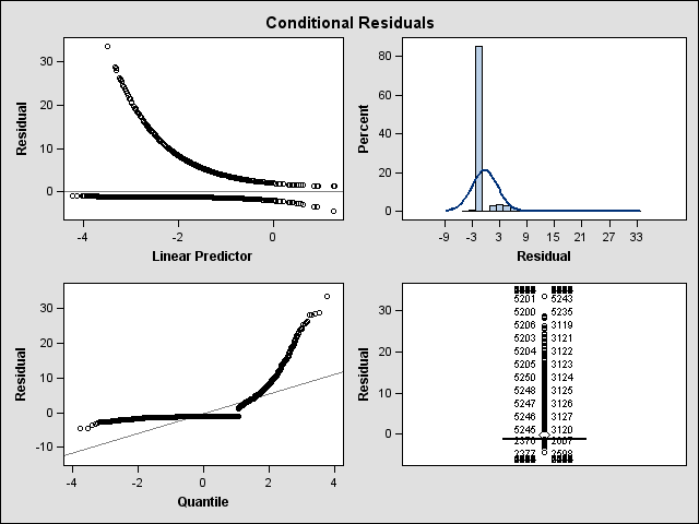
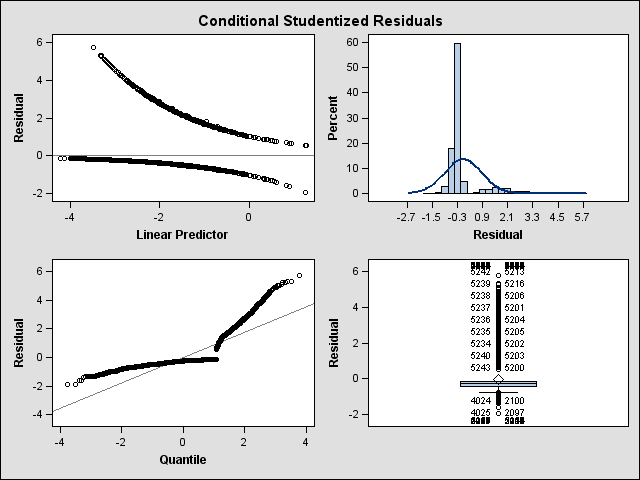
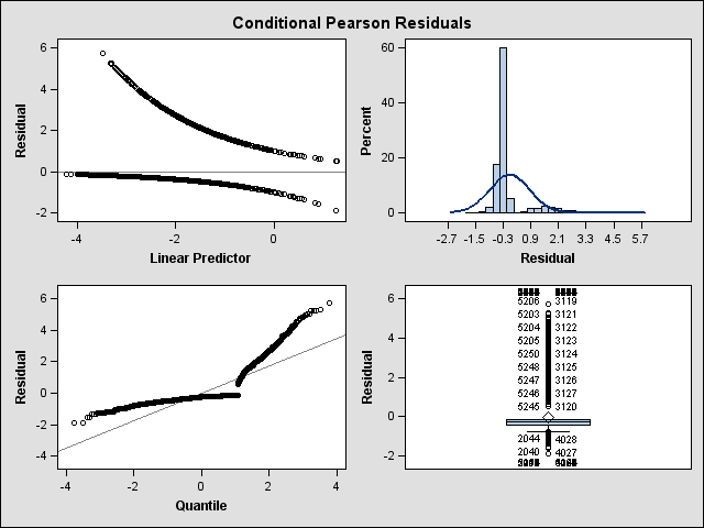
You probably have used proc glimmix in SAS 9.1.3 for analyzing multilevel data with non-normal, such as count or dichotomous outcome variables. In SAS 9.1.3, proc glimmix is an experimental procedure that requires additional downloading and installation. Now in SAS 9.2 it is a production procedure. Moreover, it offers maximum likelihood estimation wit adaptive quadrature together with Laplace approximation estimation method. Same as most of the other statistical procedures, it also provides ODS graphics, such as diagnostics graphs. It can handle normal, binary, binomial, ordered and count outcome variables.
Here is an example dealing with a binary outcome variable.
ods graphics on;
proc glimmix data = ats.thaieduc plots =(all) noclprint method=quad;
  class  sex schoolid;
  model repeat (event='1') = sex msesc sex*msesc
                            / solution dist=binary
                              oddsratio (at msesc = .5 unit msesc =.1);
  random intercept /subject = schoolid;
run;
ods graphics off;
The GLIMMIX Procedure Model Information Data Set ATS.THAIEDUC Response Variable REPEAT Response Distribution Binary Link Function Logit Variance Function Default Variance Matrix Blocked By SCHOOLID Estimation Technique Maximum Likelihood Likelihood Approximation Gauss-Hermite Quadrature Degrees of Freedom Method Containment Number of Observations Read 8582 Number of Observations Used 7516 Response Profile Ordered Total Value REPEAT Frequency 1 0 6449 2 1 1067 The GLIMMIX procedure is modeling the probability that REPEAT='1'. Dimensions G-side Cov. Parameters 1 Columns in X 6 Columns in Z per Subject 1 Subjects (Blocks in V) 356 Max Obs per Subject 41 Optimization Information Optimization Technique Dual Quasi-Newton Parameters in Optimization 5 Lower Boundaries 1 Upper Boundaries 0 Fixed Effects Not Profiled Starting From GLM estimates Quadrature Points 7 Iteration History Objective Max Iteration Restarts Evaluations Function Change Gradient 0 0 4 5507.6473045 . 130.4493 1 0 3 5482.1591394 25.48816512 24.41885 2 0 3 5479.727173 2.43196632 10.25265 3 0 3 5478.7888209 0.93835210 5.524192 4 0 2 5478.7248344 0.06398651 0.968477 5 0 3 5478.7227711 0.00206335 0.397583 6 0 3 5478.7223653 0.00040580 0.012755 7 0 3 5478.7223621 0.00000320 0.002078 Convergence criterion (GCONV=1E-8) satisfied. Fit Statistics -2 Log Likelihood 5478.72 AIC (smaller is better) 5488.72 AICC (smaller is better) 5488.73 BIC (smaller is better) 5508.10 CAIC (smaller is better) 5513.10 HQIC (smaller is better) 5496.43 Fit Statistics for Conditional Distribution -2 log L(REPEAT | r. effects) 4754.08 Pearson Chi-Square 5629.08 Pearson Chi-Square / DF 0.75 Covariance Parameter Estimates Standard Cov Parm Subject Estimate Error Intercept SCHOOLID 1.7364 0.2143 Solutions for Fixed Effects pupil Standard Effect gender Estimate Error DF t Value Pr > |t| Intercept -1.9866 0.09301 354 -21.36 <.0001 SEX 0 -0.5474 0.07603 7158 -7.20 <.0001 SEX 1 0 . . . . MSESC -0.3250 0.2328 7158 -1.40 0.1626 MSESC*SEX 0 -0.3045 0.1975 7158 -1.54 0.1232 MSESC*SEX 1 0 . . . . Odds Ratio Estimates pupil pupil 95% Confidence gender MSESC gender _MSESC Estimate DF Limits 0 0.5 1 0.5 0.497 7158 0.386 0.640 0 0.6 0 0.5 0.939 7158 0.895 0.986 1 0.6 1 0.5 0.968 7158 0.925 1.013 Type III Tests of Fixed Effects Num Den Effect DF DF F Value Pr > F SEX 1 7158 51.84 <.0001 MSESC 1 7158 4.75 0.0294 MSESC*SEX 1 7158 2.38 0.1232
-
PROC COUNTREG and PROC GENMOD for count models
Proc countreg is part of SAS/ETS for econometrics and time series. It supports the following models for count data: Poisson regression, negative binomial regression, zero-inflated Poisson (ZIP) model and zero-inflated negative binomial (ZINB) model. Proc genmod in SAS/STAT module supports everything but ZINB model. Here is a data analysis example page on zero-inflated Poisson regression model using SAS 9.2
-
PROC MCMC
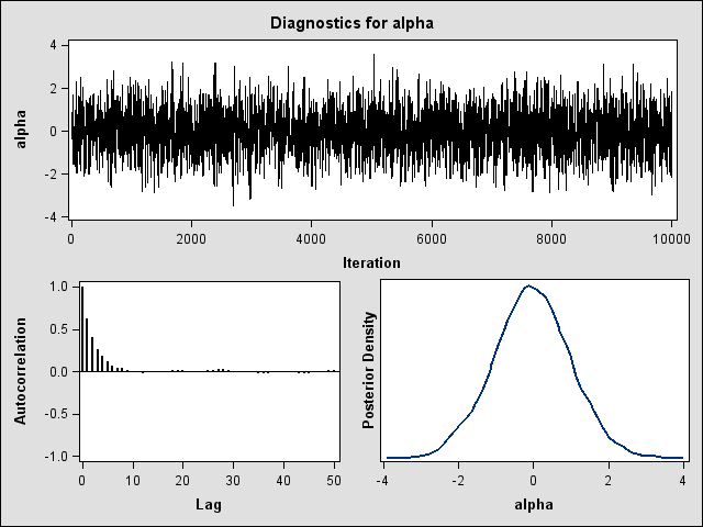
Proc mcmc is for Bayesian models using Markov chain Monte Carlo (MCMC) simulation. It can be used as a simulation tool. Here is an example from SAS documentation for simulating a normal distribution.
data x;
  run;
ods graphics on;
proc mcmc data=x outpost=simout seed=23 nmc=10000 maxtune=0
          nbi=0 statistics=(summary interval) diagnostics=none;
   parm alpha 0;
   prior alpha ~ normal(0, sd=1);
   model general(0);
run;
ods graphics off;
The MCMC Procedure Posterior Summaries Standard Percentiles Parameter N Mean Deviation 25% 50% 75% alpha 10000 -0.0392 1.0194 -0.7198 -0.0403 0.6351 Posterior Intervals Parameter Alpha Equal-Tail Interval HPD Interval alpha 0.050 -2.0746 1.9594 -2.2197 1.7869
3. New features in existing procedures
-
PROC FREQ
*testing for specified proportions;
proc freq data=ats.hsb2;
   tables ses / testp=(.33 .4 .27);
run;
The FREQ Procedure Test Cumulative Cumulative ses Frequency Percent Percent Frequency Percent -------------------------------------------------------------------- 1 47 23.50 33.00 47 23.50 2 95 47.50 40.00 142 71.00 3 58 29.00 27.00 200 100.00 Chi-Square Test for Specified Proportions ------------------------- Chi-Square 8.5785 DF 2 Pr > ChiSq 0.0137 Sample Size = 200 * distribution plot; ods graphics on; proc freq data = ats.hsb2; tables ses*prog; run; ods graphics off;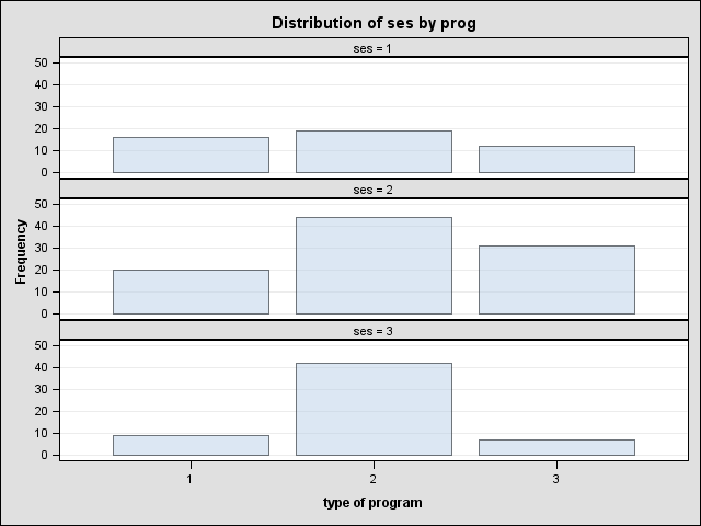 *binomial proportion test and confidence interval;
proc freq data = ats.hsb2;
tables prog /binomial (level=2 p=.55 all);
run;
*binomial proportion test and confidence interval;
proc freq data = ats.hsb2;
tables prog /binomial (level=2 p=.55 all);
run;type of program Cumulative Cumulative prog Frequency Percent Frequency Percent --------------------------------------------------------- 1 45 22.50 45 22.50 2 105 52.50 150 75.00 3 50 25.00 200 100.00 Binomial Proportion for prog = 2 ---------------------- Proportion 0.5250 ASE 0.0353 Type 95% Confidence Limits Wald 0.4558 0.5942 Wilson 0.4560 0.5931 Agresti-Coull 0.4560 0.5931 Jeffreys 0.4558 0.5934 Clopper-Pearson (Exact) 0.4534 0.5959 Test of H0: Proportion = 0.55 ASE under H0 0.0352 Z -0.7107 One-sided Pr < Z 0.2386 Two-sided Pr > |Z| 0.4773 Sample Size = 200
-
PROC REG
* robust standard error, collinearity and test of heteroscedasticity;
ods graphics on;
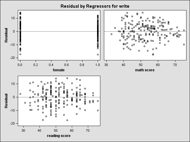
proc reg data = ats.hsb2 plots=diagnostics;
  model write = female math read /collin  spec hccmethod=1 white;
run;
quit;
ods graphics off;
The REG Procedure
Model: MODEL1
Dependent Variable: write writing score

Number of Observations Read         200
Number of Observations Used         200

                             Analysis of Variance

                                    Sum of           Mean
Source                   DF        Squares         Square    F Value    Pr > F

Model                     3     9405.34864     3135.11621      72.52    <.0001
Error                   196     8473.52636       43.23228
Corrected Total         199          17879

Root MSE              6.57513    R-Square     0.5261
Dependent Mean       52.77500    Adj R-Sq     0.5188
Coeff Var            12.45879

                              Parameter Estimates

                                   Parameter      Standard
Variable    Label           DF      Estimate         Error   t Value   Pr > |t|

Intercept   Intercept        1      11.89566       2.86285      4.16     <.0001
female                       1       5.44337       0.93500      5.82     <.0001
math        math score       1       0.39748       0.06640      5.99     <.0001
read        reading score    1       0.32524       0.06073      5.36     <.0001

                        Parameter Estimates

                                 ---Heteroscedasticity Consistent--
                                    Standard
Variable    Label           DF         Error    t Value    Pr > |t|

Intercept   Intercept        1       2.58504       4.60      <.0001
female                       1       0.94931       5.73      <.0001
math        math score       1       0.06359       6.25      <.0001
read        reading score    1       0.05874       5.54      <.0001

HCC Approximation Method: HC1

       Collinearity Diagnostics

                             Condition
  Number     Eigenvalue          Index

       1        3.58262        1.00000
       2        0.38760        3.04024
       3        0.01873       13.83149
       4        0.01105       18.00780

                      Collinearity Diagnostics

            -----------------Proportion of Variation----------------
  Number      Intercept         female           math           read

       1        0.00199        0.02429        0.00129        0.00155
       2        0.00333        0.94447        0.00305        0.00402
       3        0.90676        0.03123        0.04497        0.33778
       4        0.08791     0.00000813        0.95069        0.65665


     Test of First and Second
       Moment Specification

    DF    Chi-Square    Pr > ChiSq

     8         20.78        0.0078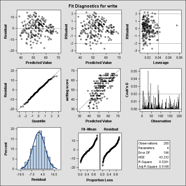
-
PROG GLM
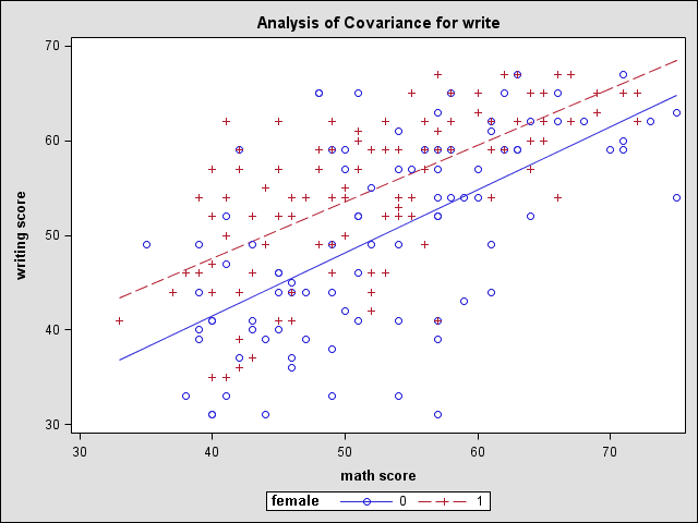
The model below has an interaction of a categorical variable with a continuous variable. SAS 9.2 creates an ANOVA plot if we just turn the ODS graphics on.
ods graphics on;
proc glm data = ats.hsb2;
  class female ;
  model write = female math female*math ;
run;
quit;
ods graphics off;
Proc glm in SAS 9.2 provides measures of effect size. Notice that this option is still experimental.
proc glm data = ats.hsb2;
  class female prog;
  model write = female prog female*prog /ss3 effectsize;
run;
quit;

                                      Sum of
Source                     DF        Squares    Mean Square   F Value   Pr > F

Model                       5     4630.36091      926.07218     13.56   <.0001

Error                     194    13248.51409       68.29131

Corrected Total           199    17878.87500

R-Square     Coeff Var      Root MSE    write Mean

0.258985      15.65866      8.263856      52.77500

           Overall Noncentrality

Min Var Unbiased Estimate    62.104
Low MSE Estimate             61.457
95% Confidence Limits        (33.709,102.7)

   Proportion of Variation Accounted for

Eta-Square                   0.26
Omega-Square                 0.24
95% Confidence Limits        (0.14,0.34)

Source                     DF    Type III SS    Mean Square   F Value   Pr > F

female                      1    1261.853291    1261.853291     18.48   <.0001
prog                        2    3274.350821    1637.175410     23.97   <.0001
female*prog                 2     325.958189     162.979094      2.39   0.0946

                                   Noncentrality Parameter

                           Min Var
                          Unbiased        Low MSE
Source                    Estimate       Estimate    95% Confidence Limits

female                       17.29           17.1        5.23     39.7
prog                         45.45           45.0       22.56     79.8
female*prog                   2.72            2.7        0.00     15.9

                               Total Variation Accounted For

                                      Semipartial
                       Semipartial         Omega-         Conservative
Source                  Eta-Square         Square    95% Confidence Limits

female                      0.0706         0.0665     0.0173  0.1469
prog                        0.1831         0.1748     0.0911  0.2718
female*prog                 0.0182         0.0106     0.0000  0.0637

                              Partial Variation Accounted For

                                          Partial
                           Partial         Omega-
Source                  Eta-Square         Square    95% Confidence Limits

female                      0.0870         0.0804     0.0255  0.1656
prog                        0.1982         0.1868     0.1014  0.2851
female*prog                 0.0240         0.0137     0.0000  0.0735
-
PROC LOGISTIC
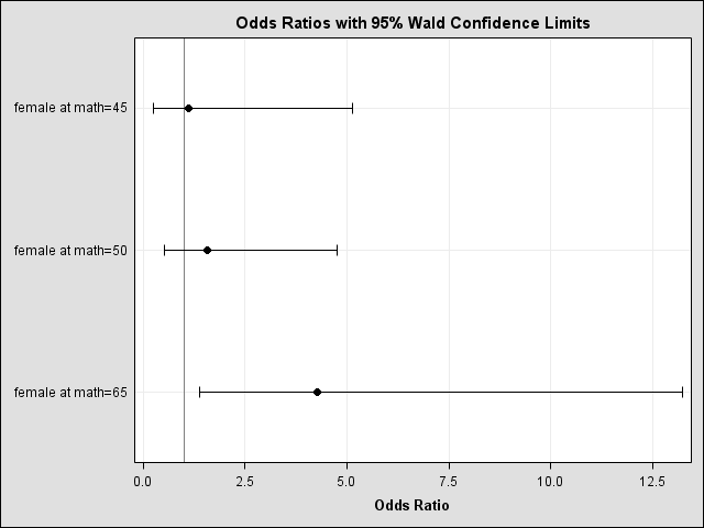
When an interaction term is present, odds ratios are calculated and graphed as shown in the example below.
data hsb2;
  set ats.hsb2;
  hon=(write>60);
run;
ods graphics on; proc logistic data = hsb2 descending; model hon = female math female*math; oddsratio female / at(math = 45 50 65); run; ods graphics off;The LOGISTIC Procedure Analysis of Maximum Likelihood Estimates Standard Wald Parameter DF Estimate Error Chi-Square Pr > ChiSq Intercept 1 -8.7458 2.1291 16.8729 <.0001 female 1 -2.8998 3.0942 0.8783 0.3487 math 1 0.1294 0.0359 12.9994 0.0003 female*math 1 0.0670 0.0535 1.5704 0.2101 Wald Confidence Interval for Odds Ratios Label Estimate 95% Confidence Limits female at math=45 1.122 0.245 5.139 female at math=50 1.568 0.517 4.759 female at math=65 4.284 1.386 13.237
When there is a quasi-complete separation of data points, the maximum likelihood estimate may not exist. SAS 9.2 provides Firth estimation for dealing with the issue of quasi or complete separation of data points.
data test;
 input Y X freq;
datalines;
0 1	3
0 2	4
0 3	5
0 3	10
1 3	6
1 4	12
1 5	8
1 6	9
1 10 11
1 11 6
;
run;
proc logistic data = test descending;
 freq freq;
  model y = x;
run;
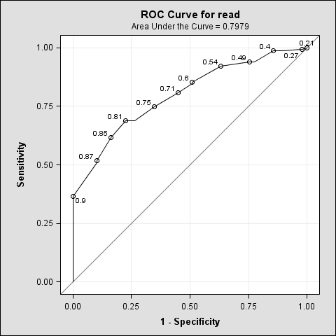
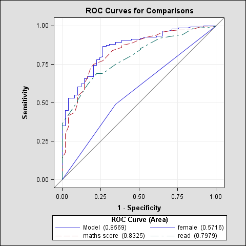
The LOGISTIC Procedure WARNING: The validity of the model fit is questionable. Testing Global Null Hypothesis: BETA=0 Test Chi-Square DF Pr > ChiSq Likelihood Ratio 64.9376 1 <.0001 Score 26.0506 1 <.0001 Wald 0.0859 1 0.7695 Analysis of Maximum Likelihood Estimates Standard Wald Parameter DF Estimate Error Chi-Square Pr > ChiSq Intercept 1 -32.8245 108.9 0.0909 0.7630 X 1 10.6361 36.2903 0.0859 0.7695 proc logistic data = test descending; freq freq; model y = x /firth; run;Testing Global Null Hypothesis: BETA=0 Test Chi-Square DF Pr > ChiSq Likelihood Ratio 57.0231 1 <.0001 Score 25.3902 1 <.0001 Wald 7.6435 1 0.0057 Analysis of Maximum Likelihood Estimates Standard Wald Parameter DF Estimate Error Chi-Square Pr > ChiSq Intercept 1 -13.0905 4.5755 8.1851 0.0042 X 1 4.0766 1.4745 7.6435 0.0057ROC curves and ROC curve contrast.
ods graphics on;
proc logistic data=hsb2 plots=roc(id=prob);
   model hon = female math read;
   roc 'female' female;
   roc 'maths score' math;
   roc 'read' read;
   roccontrast reference('female') / estimate e;
run;
ods graphics off;
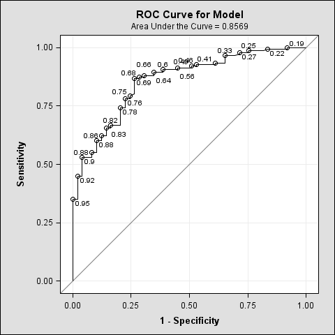
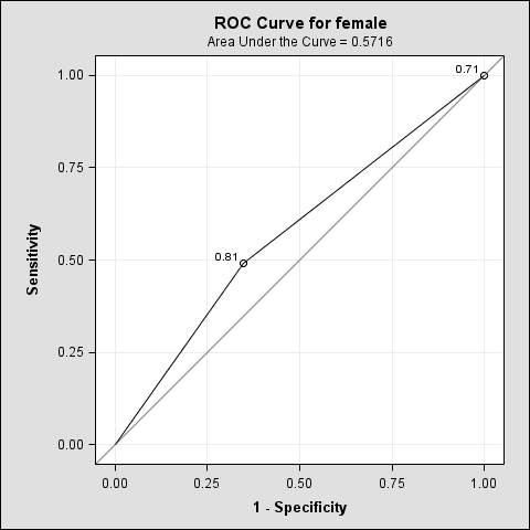
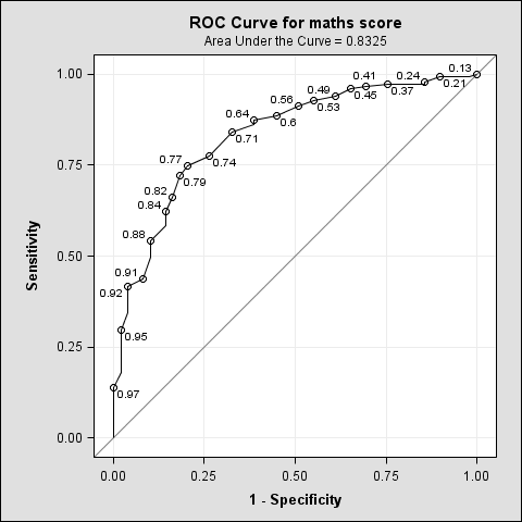
ROC Association Statistics -------------- Mann-Whitney ------------- Standard 95% Wald Somers' D ROC Model Area Error Confidence Limits (Gini) Gamma Model 0.8569 0.0288 0.8005 0.9134 0.7139 0.7142 female 0.5716 0.0400 0.4932 0.6499 0.1431 0.2880 maths score 0.8325 0.0329 0.7681 0.8970 0.6651 0.6792 read 0.7979 0.0325 0.7343 0.8616 0.5959 0.6298 ROC Association Statistics ROC Model Tau-a Model 0.2654 female 0.0532 maths score 0.2473 read 0.2216 ROC Contrast Coefficients ROC Model Row1 Row2 Row3 Model 1 0 0 female -1 -1 -1 maths score 0 1 0 read 0 0 1 ROC Contrast Test Results Contrast DF Chi-Square Pr > ChiSq Reference = female 3 113.0593 <.0001 ROC Contrast Rows Estimation and Testing Results Standard 95% Wald Pr > Contrast Estimate Error Confidence Limits Chi-Square ChiSq Model - female 0.2854 0.0439 0.1994 0.3714 42.3060 <.0001 maths score - female 0.2610 0.0532 0.1567 0.3652 24.0700 <.0001 read - female 0.2264 0.0543 0.1199 0.3329 17.3547 <.0001
4. New graphics procedures for statistical graphics
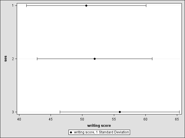
proc sgplot data=ats.hsb2;
  dot ses / response=write stat=mean
            limitstat=stddev numstd=1;
run;
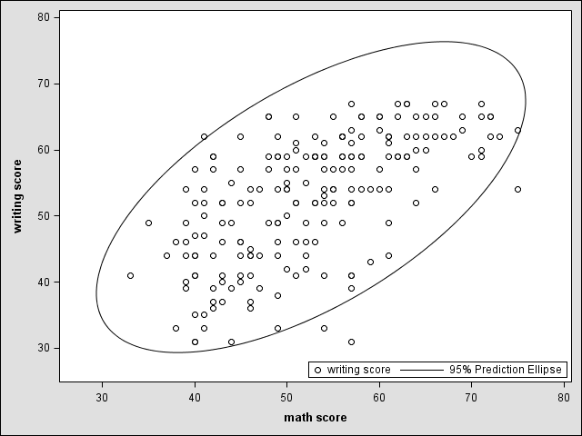
proc sgplot data=ats.hsb2;
  scatter x=math y=write;
  ellipse x=math y=write;
  keylegend / location=inside position=bottomright;
run;
title; filename odsout 'c:sastemptest.htm'; goptions device = java ; ods listing close; ods html file=odsout style=styles.ocean; proc gchart data=ats.hsb2; block prog /sumvar= write type=mean; run; ods html close; ods listing;

