NOTE: This seminar was created using SPSS version 21. Some of the syntax shown below may not work in earlier versions of SPSS.
Here are links for downloading the data files and the syntax file associated with this seminar.
- The data set called data13.sav .
- The data set called data13.xlsx .
- The data set called data13.dta .
- The data set called data13.sas7bdat .
- The data set called data13.csv .
- The SPSS syntax shown in this seminar.
Introduction
The purpose of this seminar is to help you learn about the use of SPSS syntax as an alternative to the point-and-click interface. In many instances, you may find that using syntax is simpler and more convenient than using point-and-click. The use of syntax is very useful when doing data management. One reason is because you can do repetitive tasks much quicker than you can using the point-and-click interface. You can also see what you have typed, so you don’t have to point-and-click your way back to some window to be sure that you typed the correct variable label, for example. The use of syntax is also helpful in documenting your analysis. It is difficult to take adequate notes on modifications made to the data and the procedures used to do the analyses when using the point-and-click interface. However, documenting what you are doing in a syntax file is simple, and this makes reviewing and/or reconstructing the analysis much easier.
All SPSS procedures and commands are executed using syntax, whether you use the point-and-click interface or write your own syntax. Almost everything that you can do in SPSS via point-and-click can be accomplished by writing syntax. (There are a few exceptions, most notably when using the graph editors.) Also, there are a handful of commands that are available via syntax that are not available via the point-and-click interface, such as temporary and manova. There are several ways in which you can get SPSS to show you the syntax that it is using to run your analyses, and they are explained below.
Perhaps the simplest way to ease yourself into writing SPSS syntax is to notice the syntax that SPSS includes above the results in your output file. In other words, SPSS prints the syntax of each procedure immediately above the results. If you are doing data management that does not produce results (such as creating a new variable or sorting your data), then you simply see the syntax in the output window. You can copy and paste that syntax from the output window into your syntax file so that you have a complete record of your analysis. If you would rather have the syntax go directly to the syntax file, you can click on the Paste button instead of the OK button after you have set up your analysis. This will paste the syntax that SPSS uses to run your analysis into a syntax window from which you can run the commands.
Commands in the output file If for some reason the commands are not shown in your output file, it is easy to have this done. To make this change, from the Data Editor window, click on Edit, then on Options, and then on the View tab. In the lower left-hand corner, check the option that says “Display commands in log”, and you will see all of the commands issued from then on in your output window immediately above the corresponding output.
The SPSS journal Finally, you can have the SPSS journal saved to a convenient location. The journal is a log of all of the SPSS commands that have been issued (output not included). To find or change the location of this file, from the Data Editor window, click on Edit, then Options, and under the File Locations tab, you will see where SPSS is saving the journal file. You can change that location, and you can indicate whether the journal should be overwritten every time you start SPSS, or if your next session should be appended to the bottom of the existing file. You can view the journal file using a text editor such as WordPad. Be aware that the file might be quite long, so NotePad may not be able to open the file.
How to open a new or existing syntax file To open a new syntax file, from the Data Editor window, click on File, then New, and then Syntax. If you want to open an existing syntax file, you would click on File, then Open, and then on Syntax. A syntax file is nothing more than a text file; hence, you can type commands and comments into it, and you can cut-and-paste in it as you would in any text editor. Unlike other types of SPSS files (such as data files), you can open syntax files in any text editor, such as WordPad or NotePad.
How to run (execute) syntax Now that you have commands in your syntax file, how do you run them? You have several options. You can highlight one or more commands and click on Run at the top of the syntax window. You can then select All, Selection, Current, or To End. You can highlight one or more commands (including the period at the end) and click on the right-pointing arrow at the top of the syntax editor. If you want to run only one command, you can simply put your curser anywhere in the command and click on the right-pointing arrow. SPSS while highlight and run that command. If you would rather not mouse to the top of the syntax window, you can press Ctrl-R on your keyboard (after highlighting the command or commands that you wish to run).
Multiple open data sets As of version 14, SPSS allows you to have multiple data sets open at once. The syntax that you run will be run on the “active” data set. The “active” data set is the one that is last one that you clicked on. If you get strange error messages when you run your syntax, you may have run the syntax on the wrong data file. If you did and you made changes to the data set that you did not want to make, simply close the data set without saving it. This brings up a good point: you should always work on a copy of your data, not on the original. Keep the original somewhere safe where it cannot be overwritten. If you make a mistake on the copy, it is no big deal; you just make another copy of the original and continue working on that.
SPSS has a command that allows you to control which data set is active via syntax (cleverly called dataset activate). We will explore the dateset commands later in this seminar. To keep things simple, we are going to have only one data set open at a time in this seminar.
A comment on comments One of the most important things to remember when writing SPSS syntax is that all commands must end in a period (.). This includes comments, which you can use pretty much anywhere in your syntax file. To start a comment, use either an asterisk (*) or the command comment. If you forget to end your comment with a period, SPSS will consider everything between comment or * and the next period to be part of the comment, and you may be left wondering why some of your commands did not run.
The SPSS syntax guide, AKA the SPSS Command Syntax Reference
You can access the SPSS syntax guide by clicking on “Help” and then “Command Syntax Reference” from any of the SPSS windows (the Data Editor, Syntax or Output windows). The Command Syntax Reference is a PDF that contains all of the commands available in SPSS, listed in alphabetical order. If you do not have a license for all of the SPSS add-on modules, you will not be able to run all of the commands listed. There is usually a note at the top of the entry if the command is part of a particular add-on module.
1. Opening data files
Perhaps the first thing that you need to know when using SPSS syntax is how to open a data file. The command for opening an SPSS data file is get file followed by the path where the file is located and the name of the file to be opened. The path and file name should be enclosed in quotes, and you need to include the file extension, which is .sav for SPSS data files. The .zsav data file extension was added in SPSS version 21 and denotes a compressed data file. If you have a .zsav file, you need to use SPSS version 21 or later to open the file.
get file "d:data13.sav".
If your data file is not in SPSS format, you may still be able to open it in SPSS. If you have an Excel file, you can type
get data
 /type = xlsx
 /file = 'd:datadata13.xlsx'.
Please note that there can be some issues when opening in Excel file in SPSS. One common issue is that Excel will allow you to do things that SPSS (or any other statistical package) will not. For example, you can put graphs and figures in the middle of your Excel spreadsheet, but such spreadsheets cannot be opened in SPSS. Excel allows you to use spaces in variable names, and this is not permitted in SPSS.
If your data file is in Stata format, you can type
get stata file = 'd:datadata13.dta'.
It is possible that the current version of SPSS may not be able to read in the current version of a Stata data file.
If your data file is in SAS format, you can type
get sas data = 'd:datadata13.sas7bdat'.
Please note that when using the get stata command, you need to use the file keyword. When using the get sas command, you need to use the data keyword.
SPSS can also open other kinds of files, such as .csv files. These are text files that have a comma or tab delimiter (in other words, the values of the variables are separated by either a comma or a tab). When reading a comma separated values (.csv) file into SPSS, you will need to specify the row number of the text file on which the data begin as well as the name and format of the variables in the text file.
get data
/type = txt
/file =  'd:datadata13.csv'
/delimiters = ","
/firstcase = 2
/variables =
old_var f4.2
num1 f8.2
num2 f8.2
q1 f8.2
q2 f8.2
q3 f8.2
q4 f8.2
q5 f8.2
q6 f8.2
q7 f8.2
q8 f8.2
v1 f8.2
puppy f8.2
v2 f8.2
gender f4.2.
exe.
A note about quotes You can use either single or double quotes, as shown above, as long as they match (obviously). Quotes must be used if you have spaces anywhere in your path specification or data file name, for example, “D:my dissertationmy datathe current data set.sav”. If you omit the quotes, you will get an error message, and SPSS won’t open your data file.
Password protection
Starting with SPSS version 21, you can password protect data files and output files. You can do this either through the point-and-click interface or with syntax. Syntax files cannot be password protected, so if you use syntax to set up the password protection, you (or anyone else) can see what the password is. This is not necessarily a bad thing; if you forget what the password is, the file cannot be opened. On page 1865 of the SPSS 21 Syntax Reference Guide is this: “Warning: Passwords cannot be recovered if they are lost. If the password is lost the file cannot be opened.”
The password will also be displayed in the SPSS journal file. The password is limited to 10 characters, and it is case sensitive. The password must be enclosed in quotes and can include letters, numbers, symbols and punctuation.
***Please note that password protecting a data file is not a sufficient method of protecting the confidential information of respondents. In other words, all of the rules that apply to the handling of confidential information are the same whether you use password protection or not.
Active datasets
SPSS can have many datasets open at once. If you have more than one dataset open, you need to be able to specify which dataset you want your syntax to manipulate. This can be done with the dataset commands. The dataset commands are a group of related commands that allow you to control the active dataset. This group of commands includes dataset activate, dataset close, dataset copy, dataset declare, dataset display and dataset name. Your syntax will run on the active dataset. You can make any open dataset the active dataset simply by clicking on it. When using syntax, the dataset activate command will make the listed dataset the active dataset. You may need to use the dataset name command before the dataset activate command, so that you can name the dataset that you want to make active. The name you give the dataset will not change the name of the dataset that is stored on your hard drive. We will see examples of these commands later in this presentation.
The dataset copy command is very useful for making a backup copy of your dataset. We always recommend that researchers work on a copy of their dataset and keep the original in a safe place where it cannot be lost or overwritten. If a mistake is made on the copy of the dataset, another copy can be made and the syntax that you have written can be run to bring the new copy up to date.
The new file command clears the active dataset. You may want to use this command when you are generating data within an input program.
We will start our presentation by creating some new variables. Two commands that you can use to create numeric variables are compute and if. Be aware that there is no “then” in SPSS syntax. SPSS will not create the new variables unless we issue either the execute command or a procedural command. Examples of procedural commands are list, regression and crosstabs. The procedure does not have to use the newly created variable. In many of the examples below, the execute command is technically unnecessary because we issue the procedural command list immediately afterward. (We use the list command as a convenient way of showing the output on this webpage; in practice, you would probably just look at the Data Editor window.) However, including the execute does not cause any problems, and it is handy to have in case you later change the syntax and remove the command that cause the execution of the compute commands.
In the first example, we show how to make a new variable that is a copy of a variable that already exists in the data set. We create a new variable, creatively named new_var, and set it equal to old_var. In the second example, we create a variable called newvar123 and set it equal to a constant. In our example, we set newvar123 equal to 0. At this point, every case has a value of 0 for this variable. Next, we use some if commands to change the values of newvar123 according to the values in the variables num1 and num2.
The point of the following examples is that you can make the rules for value assignments as complicated as you need them to be. You can use multiple and or or conditions in a single compute or if command. You can use either symbols or letters to specify equality or inequality. Which you use is simply a matter of personal preference. Note that spacing between variables and symbols is also a matter of preference.
| Equal to | Not equal | Less than | Less than or equal to | Greater than | Greater than or equal to | And | Or | Not |
| = | ~= <> | < | <= | > | >= | & | | | ~ |
| eq | ne | lt | le | gt | ge | and | or | not |
get file "D:Datadata13.sav".
dataset name data13.
dataset activate data13.
* making a copy of a variable: new_variable = old_variable.
compute new_var = old_var.

compute newvar123 = 0.
if num1 = 20 newvar123 = 1.
if num1 ge 50 or num2 <= 70 newvar123 = 2.
if num1=96 and num2 = 96 or num2 = 36 newvar123 = 3.
execute.
list num1 num2 old_var new_var newvar123.
    num1     num2 old_var new_var newvar123

   20.00    20.00    1.00    1.00     2.00
   20.00    30.00    2.00    2.00     2.00
   52.00    36.00    4.00    4.00     3.00
   63.00    86.00    7.00    7.00     2.00
   45.00    72.00    9.00    9.00      .
   93.00    12.00    2.00    2.00     2.00
   28.00    15.00    6.00    6.00     2.00
   75.00    46.00    5.00    5.00     2.00
   96.00    96.00    4.00    4.00     3.00
   34.00    36.00    1.00    1.00     3.00
   73.00    32.00    3.00    3.00     2.00
   20.00    30.00    3.00    3.00     2.00
   55.00    13.00    4.00    4.00     2.00
   91.00    29.00    9.00    9.00     2.00
   78.00    30.00    7.00    7.00     2.00

Number of cases read:  15    Number of cases listed:  15
You can use all sorts of math and functions when creating your variables. We will show the use of many other functions a little later in this presentation.
compute sum_num1_num2 = num1 + num2.
compute mult_num1_num2 = num1*num2.
compute div_num1 = num1/6.56.
* click on the values of div_num1 in the data editor.
execute.
list mult_num1_num2 div_num1 sum_num1_num2
 /cases from 1 to 10.
mult_num1_num2 div_num1 sum_num1_num2

    400.00        3.05       40.00
    600.00        3.05       50.00
    1872.0        7.93       88.00
    5418.0        9.60      149.00
    3240.0        6.86      117.00
    1116.0       14.18      105.00
    420.00        4.27       43.00
    3450.0       11.43      121.00
    9216.0       14.63      192.00
    1224.0        5.18       70.00

Number of cases read:  10    Number of cases listed:  10
Another point to be made involves the use of parentheses. How you use parentheses can affect the resulting variable. Notice that the two if commands below are the same, except for the use of the parentheses. The output of these two commands are put into different variables so that you can compare the results.
if num1=20 and  num2 = 96 or num2 = 30  newvar4 = 4.
if num1=20 and (num2 = 96 or num2 = 30) newvar5 = 5.
exe.
list num1 num2 newvar4 newvar5.
    num1     num2 newvar4 newvar5

   20.00    20.00     .       .
   20.00    30.00    4.00    5.00
   52.00    36.00     .       .
   63.00    86.00     .       .
   45.00    72.00     .       .
   93.00    12.00     .       .
   28.00    15.00     .       .
   75.00    46.00     .       .
   96.00    96.00     .       .
   34.00    36.00     .       .
   73.00    32.00     .       .
   20.00    30.00    4.00    5.00
   55.00    13.00     .       .
   91.00    29.00     .       .
   78.00    30.00    4.00     .

Number of cases read:  15    Number of cases listed:  15
The commands below are very similar to the commands above. The point of this example is to illustrate how SPSS processes the commands. In this example, the output of the two if commands are put into the same variable, newvar6, so that you can see what is happening.
if num1=20 and  num2 = 96 or num2 = 30  newvar6 = 4.
if num1=20 and (num2 = 96 or num2 = 30) newvar6 = 5.
exe.
list num1 num2 newvar4 newvar5 newvar6.
    num1     num2 newvar4 newvar5 newvar6

   20.00    20.00     .       .       .
   20.00    30.00    4.00    5.00    5.00
   52.00    36.00     .       .       .
   63.00    86.00     .       .       .
   45.00    72.00     .       .       .
   93.00    12.00     .       .       .
   28.00    15.00     .       .       .
   75.00    46.00     .       .       .
   96.00    96.00     .       .       .
   34.00    36.00     .       .       .
   73.00    32.00     .       .       .
   20.00    30.00    4.00    5.00    5.00
   55.00    13.00     .       .       .
   91.00    29.00     .       .       .
   78.00    30.00    4.00     .      4.00

Number of cases read:  15    Number of cases listed:  15
SPSS has many functions that can be used to create new variables. We will look at a few below. As you can see, you can use multiple functions to create a new variable.
compute nvexp = exp(num1).
compute nvlg10 = lg10(num2).
compute nvln = ln(num2).
compute nvr1 = rnd(num1, 1).
compute nvt3 = trunc(num1, 3).
compute nvrandom = rv.normal(100, 10).
compute nvlag = lag(num1).
compute nvrndmean = rnd(mean(sqrt(num1), sqrt(num2)), .01).
exe.
list nvexp nvlg10 nvln nvr1 nvt3 nvrandom num1 nvlag nvrndmean.
 nvexp nvlg10   nvln   nvr1   nvt3 nvrandom     num1  nvlag nvrndmean

5E+008   1.30   3.00  20.00  18.00   90.90     20.00    .       4.47
5E+008   1.48   3.40  20.00  18.00   99.63     20.00  20.00     4.97
4E+022   1.56   3.58  52.00  51.00   97.24     52.00  20.00     6.61
2E+027   1.93   4.45  63.00  63.00   96.40     63.00  52.00     8.61
3E+019   1.86   4.28  45.00  45.00   81.44     45.00  63.00     7.60
2E+040   1.08   2.48  93.00  93.00   82.33     93.00  45.00     6.55
1E+012   1.18   2.71  28.00  27.00   96.83     28.00  93.00     4.58
4E+032   1.66   3.83  75.00  75.00  116.34     75.00  28.00     7.72
5E+041   1.98   4.56  96.00  96.00   98.13     96.00  75.00     9.80
6E+014   1.56   3.58  34.00  33.00   96.83     34.00  96.00     5.92
5E+031   1.51   3.47  73.00  72.00   96.60     73.00  34.00     7.10
5E+008   1.48   3.40  20.00  18.00   88.40     20.00  73.00     4.97
8E+023   1.11   2.56  55.00  54.00  114.27     55.00  20.00     5.51
3E+039   1.46   3.37  91.00  90.00   91.28     91.00  55.00     7.46
7E+033   1.48   3.40  78.00  78.00   95.53     78.00  91.00     7.15

Number of cases read:  15    Number of cases listed:  15
A note on naming variables
In the preceding examples, the naming of the variables has not been terribly good. We do not suggest that you name your variables newvar1, newvar2, etc. Rather, it is good practice to name your variables something meaningful (and easy for you to type). Variable names can be up to 64 bytes long (approximately 64 characters long). However, please remember that you cannot use spaces in a variable name, and variable names should not have an underscore at the end, as these might conflict with variables created by commands or procedures. Variable names should also not end with a period, as the period is the command terminator in SPSS. (In other words, the period tells SPSS where each command ends.) You can use any combination of upper and lower case letters in a variable name, but SPSS is case insensitive. In other words, the variable name might be VarName, but you can type varname, VARname or VARNAME in the syntax, and it will work fine.
The shift values command
The shift values command was introduced in SPSS version 17. It is used to create new variables that have the shifted values of another variable in the active dataset. As you can see in the third example, you can make multiple new variables in a single call to the shift values command. Note that the keyword variable cannot be shorten to var.
shift values variable = num1 result = nvsv1 lag = 1.
shift values variable = num1 result = nvsv2 lead = 2.
shift values variable = num1 result = nvsv3 shift = -3
/variable = num1 result = nvsv4 shift = -2
/variable = num1 result = nvsv5 shift = -1.
list num1 nvsv1 to nvsv5.
    num1    nvsv1    nvsv2    nvsv3    nvsv4    nvsv5

   20.00      .      52.00      .        .        .
   20.00    20.00    63.00      .        .      20.00
   52.00    20.00    45.00      .      20.00    20.00
   63.00    52.00    93.00    20.00    20.00    52.00
   45.00    63.00    28.00    20.00    52.00    63.00
   93.00    45.00    75.00    52.00    63.00    45.00
   28.00    93.00    96.00    63.00    45.00    93.00
   75.00    28.00    34.00    45.00    93.00    28.00
   96.00    75.00    73.00    93.00    28.00    75.00
   34.00    96.00    20.00    28.00    75.00    96.00
   73.00    34.00    55.00    75.00    96.00    34.00
   20.00    73.00    91.00    96.00    34.00    73.00
   55.00    20.00    78.00    34.00    73.00    20.00
   91.00    55.00      .      73.00    20.00    55.00
   78.00    91.00      .      20.00    55.00    91.00

Number of cases read:  15    Number of cases listed:  15
The create command
The create command uses functions to make new variables. A few of these functions, such as the lag function, are available with other commands. However, create has many functions that are unique to the command. Please see our SPSS FAQ: What kinds of new variables can I make with the create command? or the Syntax Reference Guide for a list of these functions.
In the first example, we use the lag function to create the new variable nvcr1, which is num1 lagged by 1. In the next example, we create the new variables nvcr2 to nvcr5 as the lag of num1. The variable nvcr2 is lagged 2 steps, the variable nvcr3 is lagged 3 steps, and so on.
create nvcr1 = lag(num1, 1).
create nvcr2 to nvcr5 = lag(num1, 2, 5).
list num1 nvcr1 to nvcr5.
    num1    nvcr1    nvcr2    nvcr3    nvcr4    nvcr5

   20.00      .        .        .        .        .
   20.00    20.00      .        .        .        .
   52.00    20.00    20.00      .        .        .
   63.00    52.00    20.00    20.00      .        .
   45.00    63.00    52.00    20.00    20.00      .
   93.00    45.00    63.00    52.00    20.00    20.00
   28.00    93.00    45.00    63.00    52.00    20.00
   75.00    28.00    93.00    45.00    63.00    52.00
   96.00    75.00    28.00    93.00    45.00    63.00
   34.00    96.00    75.00    28.00    93.00    45.00
   73.00    34.00    96.00    75.00    28.00    93.00
   20.00    73.00    34.00    96.00    75.00    28.00
   55.00    20.00    73.00    34.00    96.00    75.00
   91.00    55.00    20.00    73.00    34.00    96.00
   78.00    91.00    55.00    20.00    73.00    34.00

Number of cases read:  15    Number of cases listed:  15
In the examples below, we use the csum and the diff functions. The csum function creates a cumulative sum, and the diff function gives the difference between values of the original variable. The degree of the difference must be specified.
create nvcr6 = csum(num2).
create nvcr7 = diff(num2, 1).
list num2 nvcr6 nvcr7.
    num2      nvcr6     nvcr7

   20.00      20.00       .
   30.00      50.00     10.00
   36.00      86.00      6.00
   86.00     172.00     50.00
   72.00     244.00    -14.00
   12.00     256.00    -60.00
   15.00     271.00      3.00
   46.00     317.00     31.00
   96.00     413.00     50.00
   36.00     449.00    -60.00
   32.00     481.00     -4.00
   30.00     511.00     -2.00
   13.00     524.00    -17.00
   29.00     553.00     16.00
   30.00     583.00      1.00

Number of cases read:  15    Number of cases listed:  15
Creating binary variables
Binary variables are variables that have only two values, 0 and 1 (and possibly missing). Here are two examples of methods that you can use to create binary variables.
compute nvbinary = (gender=2).
freq var = nvbinary.
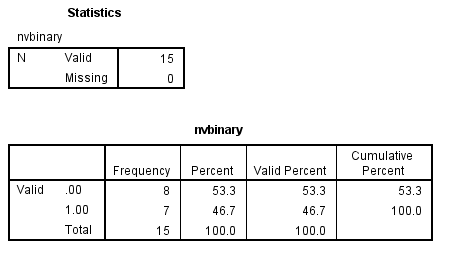
The equivalent code is presented below.
* compute nvbinary = 0.
* if gender = 2 nvbinary = 1.
* if missing(gender) nvbinary = $sysmis.
* exe.
We can use the any function to recode certain values of a variable into 1 in the new variable nvany.
compute nvany = any(num1, 20, 52, 63).
freq var = nvany.
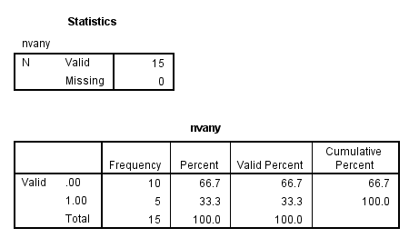
The equivalent code is presented below.
* compute nvany = 0.
* if num1 = 20 or num1 = 52 or num1 = 63 nvany = 1.
* if missing(num1) nvbinary = $sysmis.
* exe.
System variables and logical operators
System variables are variables created during your current SPSS session that contain system-required information. You can access these variables when you need to, but they don’t appear in your dataset unless you explicitly access them. All system variable names start with a dollar sign ($). There are eight system variables, but we will only mention two of them here. As we saw in the example above, you can assign system-missing values (.) with the system variable $sysmis. System missing values are considered the lowest possible value in SPSS, which you may need to know when sorting a variable that contains system missing values. In the first example below, we will use the system variable $casenum to indicate the case number.
A note about specifying missing values: When you are specifying missing values in variables that already exist in the dataset, use a function (such as missing, sysmis, etc.). When assigning a value of system missing to a variable that you are creating, use $sysmis. Also, these points are made on page 125 of the SPSS Command Syntax Reference Guide:
- “When two relations are joined with the AND operator, the logical expression can never be true if one of the relations is indeterminate. The expression can, however, be false.
- When two relations are joined with the OR operator, the logical expression can never be false if one relation returns missing. The expression, however, can be true.”
compute my_id = $casenum.
compute nvmiss = 0.
if q1 = 3 nvmiss = $sysmis.
list my_id q1 nvmiss.
 my_id       q1 nvmiss

  1.00     3.00    .
  2.00     2.00    .00
  3.00     3.00    .
  4.00     4.00    .00
  5.00    -8.00    .00
  6.00    -8.00    .00
  7.00     3.00    .
  8.00     4.00    .00
  9.00     1.00    .00
 10.00     2.00    .00
 11.00     3.00    .
 12.00     3.00    .
 13.00    -9.00    .00
 14.00      .      .00
 15.00     2.00    .00

Number of cases read:  15    Number of cases listed:  15
compute nvmiss1 = 1.
list nvmiss1.
 my_id       q1 nvmiss

  1.00     3.00    .
  2.00     2.00    .00
  3.00     3.00    .
  4.00     4.00    .00
  5.00    -8.00    .00
  6.00    -8.00    .00
  7.00     3.00    .
  8.00     4.00    .00
  9.00     1.00    .00
 10.00     2.00    .00
 11.00     3.00    .
 12.00     3.00    .
 13.00    -9.00    .00
 14.00      .      .00
 15.00     2.00    .00

Number of cases read:  15    Number of cases listed:  15
if q1 = 3 and not sysmis(q3) nvmiss1 = 2.
list q1 q2 q3 nvmiss1.
      q1       q2       q3 nvmiss1

    3.00     3.00      .      1.00
    2.00     2.00    -9.00    1.00
    3.00     1.00     2.00    2.00
    4.00     1.00     2.00    1.00
   -8.00     1.00     3.00    1.00
   -8.00     2.00     1.00    1.00
    3.00    -9.00     4.00    2.00
    4.00     4.00     2.00    1.00
    1.00     1.00     1.00    1.00
    2.00    -9.00     3.00    1.00
    3.00     3.00     2.00    2.00
    3.00     1.00     1.00    2.00
   -9.00     4.00     4.00    1.00
     .       2.00     4.00    1.00
    2.00     3.00     1.00    1.00

Number of cases read:  15    Number of cases listed:  15
if ~(sysmis(q1) and sysmis(q2) and sysmis(q3) ) nvmiss1 = $sysmis.
list q1 q2 q3 nvmiss1.
      q1       q2       q3 nvmiss1

    3.00     3.00      .       .
    2.00     2.00    -9.00     .
    3.00     1.00     2.00     .
    4.00     1.00     2.00     .
   -8.00     1.00     3.00     .
   -8.00     2.00     1.00     .
    3.00    -9.00     4.00     .
    4.00     4.00     2.00     .
    1.00     1.00     1.00     .
    2.00    -9.00     3.00     .
    3.00     3.00     2.00     .
    3.00     1.00     1.00     .
   -9.00     4.00     4.00     .
     .       2.00     4.00     .
    2.00     3.00     1.00     .

Number of cases read:  15    Number of cases listed:  15
compute nvmiss2 = 1.
if ~(sysmis(q1) | sysmis(q2) | sysmis(q3) ) nvmiss2 = $sysmis.
list q1 q2 q3 nvmiss1 nvmiss2.
      q1       q2       q3 nvmiss1 nvmiss2

    3.00     3.00      .       .      1.00
    2.00     2.00    -9.00     .       .
    3.00     1.00     2.00     .       .
    4.00     1.00     2.00     .       .
   -8.00     1.00     3.00     .       .
   -8.00     2.00     1.00     .       .
    3.00    -9.00     4.00     .       .
    4.00     4.00     2.00     .       .
    1.00     1.00     1.00     .       .
    2.00    -9.00     3.00     .       .
    3.00     3.00     2.00     .       .
    3.00     1.00     1.00     .       .
   -9.00     4.00     4.00     .       .
     .       2.00     4.00     .      1.00
    2.00     3.00     1.00     .       .

Number of cases read:  15    Number of cases listed:  15
The numeric command
The numeric command allows you to specify the format of the new variable. The numeric command creates an empty variable that you then populate using another command, such as the compute or if command. In the first example below, we create a numeric variable called nvn1. Because we did not list a format on the numeric command, this variable has the default format, which is f8.2. This means that the variable has a length of 8, with 2 spaces after the decimal, 1 space for the decimal, and 5 spaces for integer portion of the number. In the second call to the numeric command, we create two new variables, nvn2 and nvn3. These two variables have different formats. The three compute commands populate our three new variables.
numeric nvn1.
numeric nvn2 (f4.0) nvn3 (f8.4).
compute nvn1 = q1.
compute nvn2 = q1.
compute nvn3 = q1.
exe.
list q1 nvn1 nvn2 nvn3.
      q1   nvn1 nvn2     nvn3

    3.00   3.00    3   3.0000
    2.00   2.00    2   2.0000
    3.00   3.00    3   3.0000
    4.00   4.00    4   4.0000
   -8.00  -8.00   -8  -8.0000
   -8.00  -8.00   -8  -8.0000
    3.00   3.00    3   3.0000
    4.00   4.00    4   4.0000
    1.00   1.00    1   1.0000
    2.00   2.00    2   2.0000
    3.00   3.00    3   3.0000
    3.00   3.00    3   3.0000
   -9.00  -9.00   -9  -9.0000
     .      .      .    .
    2.00   2.00    2   2.0000

Number of cases read:  15    Number of cases listed:  15
This brings up the topic of changing numeric formats, which can be done with the formats command.
formats num1 (dollar6) num2 (f4.1).
exe.
list num1 num2.
  num1 num2

   $20 20.0
   $20 30.0
   $52 36.0
   $63 86.0
   $45 72.0
   $93 12.0
   $28 15.0
   $75 46.0
   $96 96.0
   $34 36.0
   $73 32.0
   $20 30.0
   $55 13.0
   $91 29.0
   $78 30.0

Number of cases read:  15    Number of cases listed:  15
The formats command only works with numeric variables. This command does not change how many decimal places you see in tables in your output (the only output modified by this command is the output for the list command), and it does not change the actual values used by SPSS when doing computations. However, it can be very useful when making graphs with the ggraph command and GPL. Please see Making Graphs with the ggraph command and GPL for more information and examples.
Creating standardized variables
Creating standardized variables in SPSS is very simple. You can use the descriptives command with the save subcommand. If you want to name the new standardized variable instead of using the SPSS default name, you can put that name in parentheses after the variable you wish to standardize. You can also create multiple standardized variables in a single call to descriptives.
descriptives num1
 /save.
desc num1 (num1z)
 /save.
desc q1 (q1z) q2 (q2z) q5 (q5z)
 /save.
Note that a variable label was automatically created for the new variables. We also see that the command descriptives is another command name that can be shortened (to desc).

The keyword “to”
SPSS uses special “keywords” to identify commands, subcommands, functions operators and other specifications. Some of the keywords that we will use in this presentation include to, all and thru.
When creating variables, the SPSS keyword to will create variables with consecutive numbering. When using to in syntax to refer to variables that already exist in the data set, SPSS assumes that variables are sequential, or positionally consecutive (all variables between the first variable listed and the last variable listed in the command will be included). There are some commands in SPSS that will use the keyword to in both a positionally and a numerically consecutive manner, depending on whether existing variables are being modified in some way or whether new variables are being created. Some of these commands include autorecode, recode, aggregate and rename variables.
autorecode v1 to v2 /into nvar1 to nvar3.
rename variables (q6 to q8 = q16 to q18).
compute nvmean5 = mean(q1 to q5).
exe.
list v1 to v2 nvar1 to nvar3 q16 to q18 nvmean5.
      v1    puppy       v2 nvar1 nvar2 nvar3    q16    q17    q18 nvmean5

    7.00     5.00     2.00   7     4     2     9.00  10.00   7.00    2.67
    8.00     9.00     3.00   8     8     3     6.00  11.00   5.00   -1.00
    5.00     6.00     6.00   5     5     6     3.00  16.00   3.00    2.25
    3.00     3.00     9.00   3     3     9     8.00  15.00   9.00    -.50
    2.00     1.00     8.00   2     1     8     5.00  11.00   5.00    -.50
    6.00     2.00     8.00   6     2     8     2.00  14.00   1.00   -3.50
    9.00     5.00     7.00   9     4     7     7.00  17.00   8.00     .00
    4.00     7.00     5.00   4     6     5     5.00  18.00   5.00    3.25
    1.00     8.00     4.00   1     7     4     2.00  12.00   2.00    1.00
    8.00     7.00     2.00   8     6     2     1.00  14.00   9.00    -.50
    5.00     3.00     1.00   5     3     1     4.00  19.00   6.00    3.25
    7.00     9.00     3.00   7     8     3     7.00  15.00   3.00    2.00
    4.00     6.00     6.00   4     5     6     8.00  16.00   7.00     .25
    1.00     5.00     8.00   1     4     8     5.00  15.00   4.00    2.33
    2.00     1.00     7.00   2     1     7     2.00  17.00   1.00    2.50


Number of cases read:  15    Number of cases listed:  15
Renaming variables
The rename variables command does exactly what you think it does: it renames variables. If you rename more than one variable at a time, you may need to use parentheses. You can also use this command to exchange variable names, as shown in the third example.
rename variables nvbinary = female.
* parentheses are optional.
rename variables (q16 = q6) (q17 = q7) (q18 = q8).
* parentheses not optional.
rename variables (q6 q7 q8 = q16 q17 q18).
* exchanging variable names.
rename variables (q16 = q18) (q18 = q16).
Recoding variables
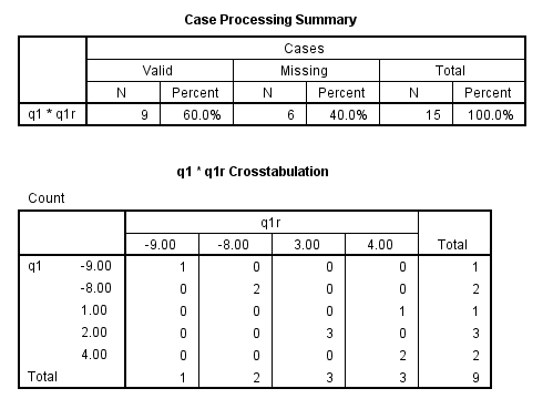
The recode command recodes the values of either numeric or string variables. There are several input keywords that you can use with this command, including lo, lowest, hi, highest, thru, missing, sysmis and else. The keyword thru includes the specified end value. The keywords lowest and highest (and lo and hi) include user-defined missing but not system-missing values. The keyword missing specifies both user-defined missing and system missing, while the keyword sysmis only specifies system-missing. Output keywords include copy and sysmis. There are other keywords that can be used when recoding string variables, but we will not cover those here.
recode q1 (1 = 4) ( 2 = 3) (3 = sysmis) (else = copy) into q1r.
crosstabs
/tables = q1 by q1r.
list q1 q1r.
      q1    q1r

    3.00    .
    2.00   3.00
    3.00    .
    4.00   4.00
   -8.00  -8.00
   -8.00  -8.00
    3.00    .
    4.00   4.00
    1.00   4.00
    2.00   3.00
    3.00    .
    3.00    .
   -9.00  -9.00
     .      .
    2.00   3.00

Number of cases read:  15    Number of cases listed:  15
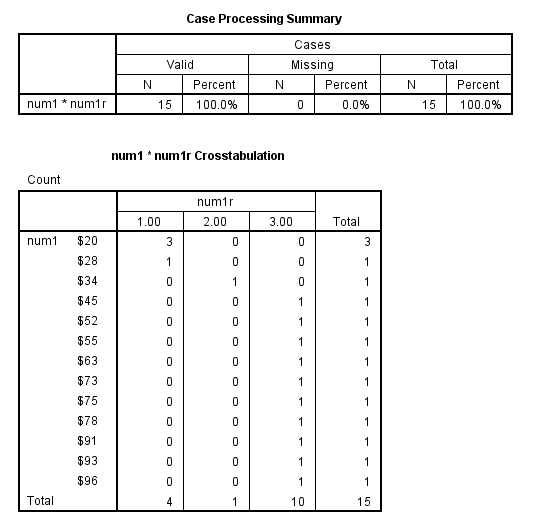
recode num1 (lowest thru 30 = 1) (31 thru 40 = 2) (41 thru hi = 3) (missing = -9) into num1r.
crosstabs num1 by num1r.
formats num1 (f8.2).
list num1 num1r.
    num1  num1r

   20.00   1.00
   20.00   1.00
   52.00   3.00
   63.00   3.00
   45.00   3.00
   93.00   3.00
   28.00   1.00
   75.00   3.00
   96.00   3.00
   34.00   2.00
   73.00   3.00
   20.00   1.00
   55.00   3.00
   91.00   3.00
   78.00   3.00

Number of cases read:  15    Number of cases listed:  15
Delete variables
The delete variables command is a very handy command, but obviously, this command needs to be used with caution. The delete variables command was introduced in SPSS version 12.
delete variables num1r q1r.
Another way to do the same thing is to use the save outfile command with either the keep or the drop subcommand. The difference is that with the delete variables command, you are not saving a new data file.
save outfile "D:DataSeminarsSPSS Syntax Seminar2013 updatedata13_deleted.sav"
/drop num1r q1r.
Variable level
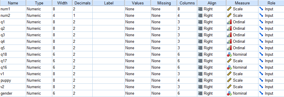
The variable levels are shown in the Variable View window of the Data Editor in the second column from the right. With earlier versions of SPSS, the only procedure that used the variable level was igraph, which is now a deprecated graphing command. However, in more recent versions of SPSS, other procedures are making use of the variable levels, so it is becoming more important that users know how to modify them. Here is a simple example.
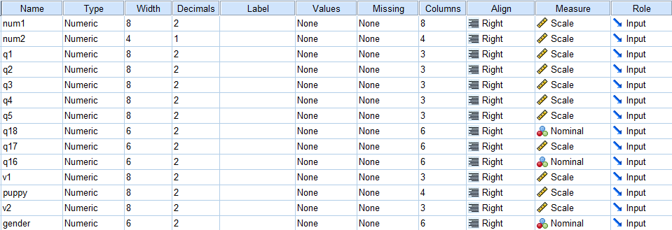
variable level num1 num2 (scale)
/q1 to q5 (ordinal)
/gender (nominal).
Variable role
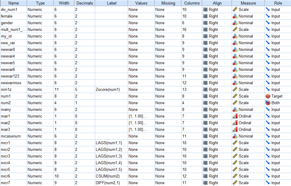
The variable role command was introduced in SPSS version 18, and it is used with some of the commands that were introduced in that and later versions of SPSS. Some of the roles a variable can take include input (independent variable), target (dependent variable), both and none. The specified role does not matter when you are writing syntax, but it does matter when you are using the point-and-click interface. This command is mentioned in our seminar on SPSS syntax because we realize that many people will use the point-and-click interface to help them get a template of the syntax for a procedure, and it can be confusing when some variables appear in some dialog boxes and not others.
variable role
/target num1
/input q1 to q5
/both num2.

Sorting variables
The sort variables command was introduced in SPSS version 16. You can sort the variables in your dataset by name, type, format, label, values, missing, measure, role, columns, alignment, and attribute. Sorting variables is a good way to make sure that you have done all of the data documenting that you meant to do (by sorting the variables by labels or values, for example). We will cover the topic of documenting data shortly.
sort variables by type.
sort variables by role.
sort variables by name.
User-defined missing values
There are two different types of missing data in SPSS: system-missing and user-defined missing. System-missing is displayed as a dot (.) in the column of a numeric variable. System missing values are considered the lowest possible value in SPSS. You can define your own missing values, which are called user-defined missing for numeric variables. Although displayed differently, both system-missing and user-defined missing values are just missing values to SPSS, and they are treated the same way (except in filter variables, see below). Both will be deleted from analyses that call for listwise deletion. The only “difference” is that they will be displayed in separate categories in crosstabs, frequencies, etc.
There are some keywords that can be used with numeric value lists, and they include lo, lowest, hi, highest and thru.
missing values q1 to q5 (-9).
missing values q3 (-7 thru hi, -999).

You can declare, change or clear missing values by issuing the missing values command again. To clear all missing values, simply leave the parentheses empty.
missing values q1 (-9 -8).
missing values q5 ().

It is important to realize is that you can create the same variable in different ways, and that the missing values may be handled differently. Note that above we defined -8 and -9 as missing values for the variable q1 (in the third missing values command), and -9 as a missing value for the variable q2 (in the first missing values command).
compute nvmiss1 = q1 + q2.
compute nvmiss2 = sum(q1, q2).
exe.
list q1 q2 nvmiss1 nvmiss2.
      q1       q2 nvmiss1 nvmiss2

    3.00     3.00    6.00    6.00
    2.00     2.00    4.00    4.00
    3.00     1.00    4.00    4.00
    4.00     1.00    5.00    5.00
   -8.00     1.00     .      1.00
   -8.00     2.00     .      2.00
    3.00    -9.00     .      3.00
    4.00     4.00    8.00    8.00
    1.00     1.00    2.00    2.00
    2.00    -9.00     .      2.00
    3.00     3.00    6.00    6.00
    3.00     1.00    4.00    4.00
   -9.00     4.00     .      4.00
     .       2.00     .      2.00
    2.00     3.00    5.00    5.00

Number of cases read:  15    Number of cases listed:  15
Documenting data
There are many ways to document your data using SPSS. We have already covered some of these topics, and we will discuss some others shortly.
- create document
- label data file
- label variables
- label values of variables
- user-defined missing
- create variable attributes
- create datafile attributes
- set variable role
- set variable level
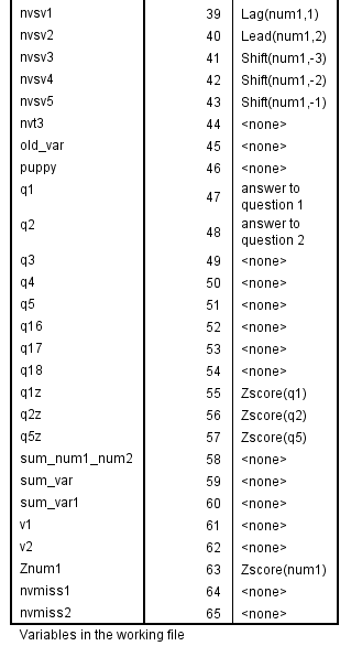
You can view the documentation that you have created using the sysfile info and display commands. When using the sysfile info command, you must specify the file path. Also, the maximum length of a variable label is 255 characters and the maximum length of a value label is 120 bytes (approximately 120 characters). The display command allows you to display certain information about the dataset and the variables within it. For example, you can display all of the variable names, documents, dictionary information, attributes, labels, scratch variables, vector names and macros.
Let’s look at some of the commands that we can use to archive information about our data file.
The document command is very handy and allows you to keep notes with your data set. You can use the document drop command to remove a document from your data file. The add document command can be used to include additional notes to your document. Unlike the document command, you will need to use quotes around each line of the text when using this command.
The file label command is used to label the data file itself. This is particularly useful when you have multiple copies of a data set that are slightly different.
The variable labels command allows you to assign labels to your variables. Doing so is an important part of developing a codebook. We strongly recommend that all data sets have a codebook, even if the researcher is not planning on sharing the data with others. The codebook reminds you of all of the details of your data set, which is important when you have to come back to the data at a later time.
The value labels command allows you to assign labels to the values of a variable. You can use the add value labels command to labels values that were not labeled with the value labels command.
sysfile info "D:DataSeminarsSPSS Syntax Seminar2013 updatedata13_doc.sav".
document These data were collected from January 13, 2012 through June 20, 2012.
add document "this is my additional comment"
"to my original document command.  Note "
"that each additional line of text must be enclosed in quotes.".
display document.
* drop documents.
file label SPSS Syntax Seminar Part 1 data file.
save outfile "D:DataSeminarsSPSS Syntax Seminar2013 updatedata13_doc2.sav".
sysfile info "D:DataSeminarsSPSS Syntax Seminar2013 updatedata13_doc2.sav".
variable labels q1 "answer to question 1"
q2 "answer to question 2".
display labels.
value labels q1 to q3 q5 1 'strongly disagree' 2 'disagree' 3 'agree'.
add value labels q5 4 'strongly agree' 5 'not applicable'.
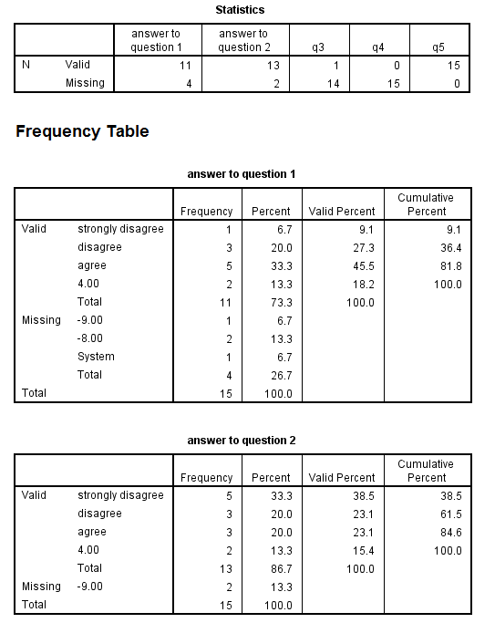
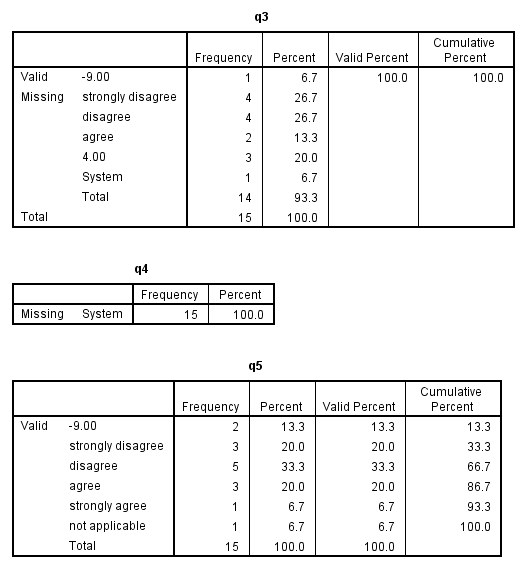
freq var = q1 to q5.
save outfile "D:Datadata13_doc3.sav".
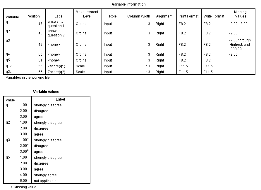
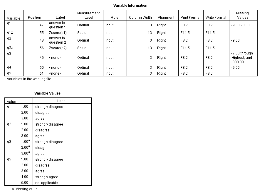
display dictionary
/variables = q1 to q5 q1z q2z.
display sorted dictionary
variables = q1 to q5 q1z q2z.
The variable attribute command
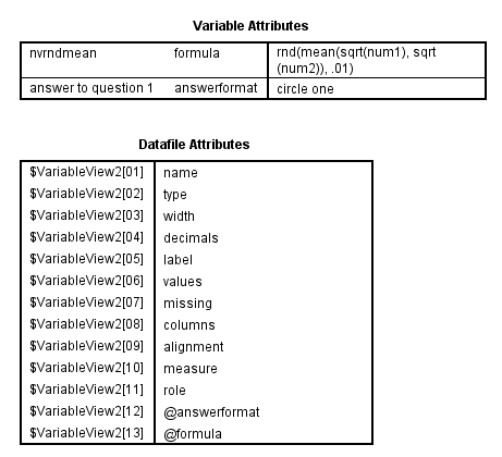
The variable attribute command was introduced in SPSS version 14 and allows users to assign attributes to variables in the active dataset. The attributes are saved with the data dictionary. In the examples below, we assign attributes that tell us what type of response was required for q1 and what formula was used to create the variable nvrndmean. This type of information is important to keep with the dataset, especially if the written code book becomes lost.
variable attribute
variables = q1
attribute = answerformat('circle one')
/variables = nvrndmean
attribute = formula('rnd(mean(sqrt(num1), sqrt(num2)), .01)' ).
display attributes.
The datafile attribute command
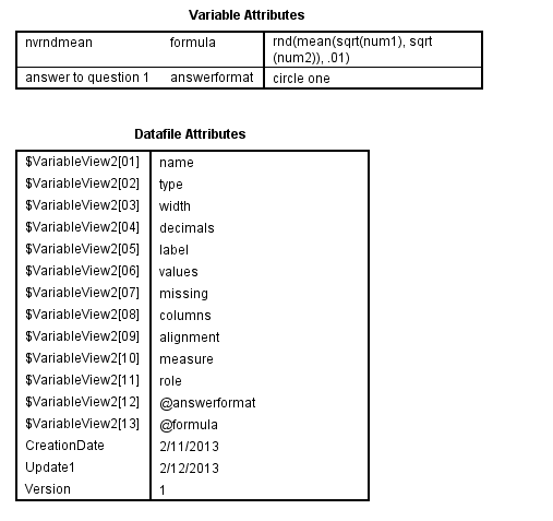
The datafile attribute command is similar to the variable attribute command, but, of course, it sets attributes for the data file. The delete keyword allows attributes to be removed.
datafile attribute
attribute = Version ('1')
                CreationDate ('2/11/2013')
                Update1('2/12/2013').
display attributes.
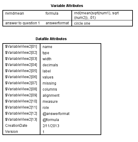
datafile attribute
delete = Update1.
display attributes.
The codebook command
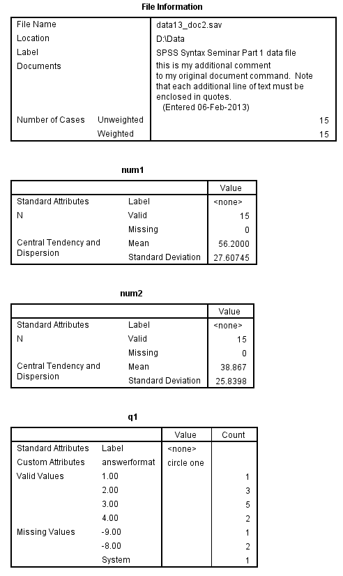
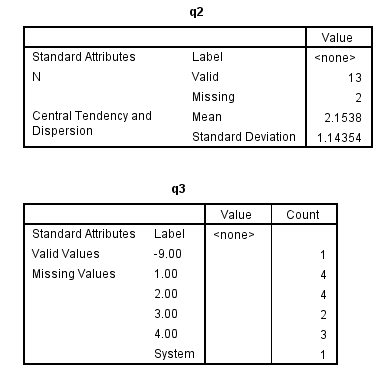
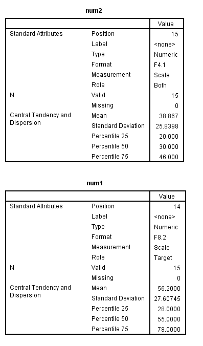
The codebook command was introduced in SPSS version 17 and updated in version 18. The codebook command displays dictionary information and summary statistics for variables in the active dataset. For nominal and ordinal variables, summary statistics include counts and percents. For scale (continuous) variables, the mean, standard deviation and quartiles are displayed. The split file status of the dataset is ignored, but the filter status is honored for computing summary statistics.
In the interest of saving space, only part of the output from the first codebook command is shown.
codebook num1 num2 q1 to q3
/varinfo label valuelabels missing attributes
/statistics count mean stddev
/fileinfo name location label documents casecount.
codebook num1 num2
/options maxcats = 5 sort = descending.
Subsetting data using the split file, filter and select if commands
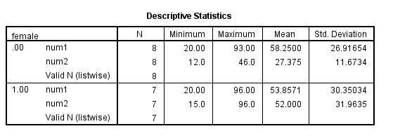
Up to now, we have been focusing mostly on data management. However, the reason researchers do data management is to prepare the data for analysis, and we will see some descriptive statistics shortly. First, though, let’s talk about subsetting data. There are several different ways that you can do this in SPSS. Perhaps the simplest way is to have SPSS run the same analysis for each level of a categorical variable. In our sample dataset, let’s say that we want to get the mean of some variables for each level of the variable gender. We will use the split file command to do this. Before we can issue this command, we will need to sort the data by gender.
If we had any missing values on the variable gender, our output would be broken into three sections: one for missing values of gender, one for gender = 1 and one for gender = 2.
sort cases by female.
split file by female.
desc num1 num2.
split file off.
desc num1 num2.
Sometimes you want the analysis only for one gender, not both. Of course, you could use the split file command and only look at the output for the gender of interest, but if your analysis takes a long time to run, this can be a problem. There are at least two ways to analyze only one subset of your data. You can use a filter or you can keep only the cases that you want to analyze in your dataset. Usually, researchers prefer to create and use a filter rather than eliminate cases from the dataset. To filter cases in SPSS, you need a binary variable (a variable that only has the values 0 and 1) and use that variable with the filter command. Only the cases coded as 1 will be included in the analyses; the cases coded as 0 (or missing) will not. The filter command will stay in effect until you “turn it off” with the filter off command (or the use all command). You can look in the lower right corner of the SPSS data window to see if a filter is on.
filter by female.
desc num1 num2.
filter off.
* use all.
desc num1 num2.
You can permanently delete cases from your dataset with the select if command. Cases coded as 1 will remain in your dataset; cases coded as 0 (or missing) will be deleted from the dataset. Once you run the select if command, you will not be able to recover the cases that were deleted. If you delete cases that you did not intend to delete, close the data file without saving it and reopen the data file.
We do not want to permanently delete any cases from our sample data file, so we will put the temporary command before the select if command. The temporary command is available only via syntax (not through the point-and-click menu system). The temporary command stays in effect only until the next executable command is executed. That is why the output for the first list command (which is the first executable command after temporary) has only seven observations (the seven that met the criteria listed on the select if command), while the second list command includes all of the observations from our data set. Although for this seminar we only use the temporary command while subsetting, it has many other uses.
temporary.
select if (gender = "f" and q1 ge 2).
list num1.
    num1

   20.00
   20.00
   52.00
   93.00
   75.00
   73.00
   55.00
   78.00

Number of cases read:  8    Number of cases listed:  8
list num1.
    num1

   20.00
   20.00
   52.00
   93.00
   75.00
   73.00
   55.00
   78.00
   63.00
   45.00
   28.00
   96.00
   34.00
   20.00
   91.00

Number of cases read:  15    Number of cases listed:  15
The n of cases command
Another way to use only part of your data is to use the n of cases command. This command will limit the number of cases in the active dataset to N cases (of course, you decide what N will be). This command is especially handy when you have a very large dataset, you are debugging your syntax and running a command takes longer than you would like. You can simply limit the number of cases such that your commands run quickly, so that you can see if you get any error messages, if you have all of the desired options specified, etc. We will use the temporary command with the n of cases command in the examples below.
Also note how the n of cases works with the sample and select if commands: “If N OF CASES is used with SAMPLE or SELECT IF, the program reads as many records as required to build the specified n cases. It makes no difference whether N OF CASES precedes or follows SAMPLE or SELECT IF” (page 1363).
temporary.
n of cases 3.
list my_id num1.
 my_id     num1

  1.00    20.00
  2.00    20.00
  3.00    52.00

Number of cases read:  3    Number of cases listed:  3
temporary.
n of cases 3.
select if female = 1.
list my_id female num1.
 my_id female     num1

  4.00   1.00    63.00
  5.00   1.00    45.00
  7.00   1.00    28.00

Number of cases read:  3    Number of cases listed:  3
list my_id female num1.
 my_id female     num1

  1.00    .00    20.00
  2.00    .00    20.00
  3.00    .00    52.00
  4.00   1.00    63.00
  5.00   1.00    45.00
  6.00    .00    93.00
  7.00   1.00    28.00
  8.00    .00    75.00
  9.00   1.00    96.00
 10.00   1.00    34.00
 11.00    .00    73.00
 12.00   1.00    20.00
 13.00    .00    55.00
 14.00   1.00    91.00
 15.00    .00    78.00

Number of cases read:  15    Number of cases listed:  15
The sample command
You can also use the sample command to limit the number of cases in the active dataset. This command can be used in two ways. You can specify the proportion of cases you want to keep in the active dataset (by giving a decimal value between 0 and 1), or you can specify the number of cases (n) to be sampled from a specific number of cases (m). You may want to set the seed before running the sample command, as it uses a pseudo-random number generator to select the cases. If you want to get the same cases each time you run the command, you will need to set the seed.
set seed 1326.
temporary.
sample .5.
list my_id num1.
 my_id     num1

  2.00    20.00
  6.00    93.00
  7.00    28.00
 14.00    91.00

Number of cases read:  4    Number of cases listed:  4
If you specify m less than the actual number of cases in the active dataset, the sample will be drawn only from the first m cases. If you specify m greater than the number of cases in the active dataset, the sample will be an equivalent proportion of cases from the active dataset. Hence, in our second example, we sample 4 cases from 20, but we only have 15 cases in our active dataset. Four cases out of 20 is 4/20 = .2, and .2 proportion of 15 cases is 3.
set seed 1472.
temporary.
sample 4 from 10.
list my_id num1.
 my_id     num1

  1.00    20.00
  3.00    52.00
  7.00    28.00
  8.00    75.00

Number of cases read:  4    Number of cases listed:  4
set seed 159122.
temporary.
sample 4 from 20.
list my_id num1.
 my_id     num1

  6.00    93.00
  8.00    75.00
 10.00    34.00

Number of cases read:  3    Number of cases listed:  3
The output commands
Just as there is a group of dataset commands, so there is a group of output commands. These commands allow you to control output files via syntax. The group of output commands includes output activate, output close, output display, output export, output name, output new, output open and output save.
The Output Management System (OMS)
In addition to controlling output files, you can control parts of the output from a procedure. This is done with the Output Management System, or OMS. OMS is particularly useful when you need to get one or more specific values from an output and use those in the next step of your analysis or program. For example, you may want to capture the regression coefficients from one model and use them with a different data set. The group of OMS commands includes oms, omsend, omsinfo and omslog. We have some examples using the OMS commands at SPSS FAQ: How can I output my results to a data file in SPSS? and SPSS FAQ: How can I use aggregate and OMS to help explain a three-way interaction in ANOVA? .
Saving SPSS files
You can save your SPSS data files with the save outfile command. All you need after the command is the file path and the name of the new data set.
save outfile "D:datanew_data13.sav".
There are several handy subcommands that you can use when saving your data file. For example, you can use the keep subcommand. As you would expect, you list the variables that you want to save in the new data set on the keep subcommand. You can order them in any order that you want them in the new data set. In this example, we move the variables gender, num1 and num2 so that they are the first variables in the new data set (called my_data13.sav), and then we keep all of the other variables in the order in which they appear in the old data set (data13.sav) by using the SPSS keyword all. If you want to delete a few variables from the new data set, you can use the drop subcommand and list the variables that should not be included in the new data set (no example shown). If you want to delete cases from the saved dataset, you can filter your data file and use the unselected subcommand to delete the filtered cases.
save outfile "D:datamy_data13_keep.sav"
/keep = gender num1 num2 all.

filter by female.
save outfile "D:datamy_data13_female.sav"
/unselected = delete.
You can also save your data file in different formats. In the example below, we save our data file in Stata format. Please note that as of SPSS version 21, SPSS can save data in Stata versions 4 through 8 (Stata version 8 is the default). This is usually not a problem, because the current version of Stata can read Stata 8 data files. Also, keep in mind that SPSS data files can have many more variables than a Stata Intercooled data file can have (the limit in Stata IC is 2048). This means that you may need to delete some variables from your SPSS data file before running the save translate command.
save translate outfile = "D:Datamy_data13.dta"
/version = 8
/type = stata
/edition = intercooled.
Here is an example of saving an SPSS data file as a SAS version 9 data file.
save translate outfile = "D:datamy_data13.sas7bdat"
/valfile = "D:datalabels.sas"
/version = 9
/platform = windows
/replace.
In the first example below, we save our SPSS data file as a comma separated values (.csv) file without the variable names at the top of the file. This is good for making an Mplus data file. In the second example, we include the variable names at the top of the file and use the value labels instead of the data values.
* saving a comma separated values file without variable names at the top.
* good for making Mplus data files.
save translate outfile = "D:datamy_data13_nonames.csv"
/type = csv.

* csv file with names at the top and labels.
save translate outfile = "D:datamy_data13_names.csv"
/type = csv
/fieldnames
/cells = labels.
If you want want to save your output file, you can use the output export command. Please see our FAQ on this.
SPSS output files have the file extension .spv. You can also save output files with the .spw extension, which is for the SPSS Web Reports format. Older SPSS output files may have the extension .spo. These files can be read with the SPSS Smart Viewer, which can be downloaded for free from the IBM SPSS website. Note that only .spo files that were created using a Windows machine can be read with the SPSS Smart Viewer.
You can save SPSS syntax files. They have an .sps extension. SPSS syntax files are simply text files, so they can be opened and read in any text editor. Despite much wishful thinking, there is no command to translate your SPSS syntax files into SAS or Stata syntax files. Sorry.
The erase command
You can remove files from your computer by using the erase command. You can remove only one file at a time with this command, and wildcard characters are not permitted. You can remove files created by SPSS as well as files not created by SPSS. As noted on page 701 of the Syntax Reference Guide: “Use ERASE with caution.” Obviously, this is very good advice. Below is an example.
erase file = "D:datamy_data13_names.csv".
Pasting syntax
When using the point-and-click interface in SPSS, you have the choice of clicking on OK or Paste once you have set up your analysis or data management command. If you click on Paste, SPSS will put the syntax for that command in your syntax file without running it. This can be a useful way to learn SPSS syntax, but be aware that you may see much more syntax than you actually need to run a command. Also note that SPSS uses capitalization to show which words are part of the SPSS syntax and which are supplied by the user (such as variable names). As we mentioned before, SPSS is not case sensitive, so there is no need to type SPSS command names, subcommand names or keywords in capital letters if you rather not. Let’s look at one example.
Notice that we get exactly the same output using both of the examine commands shown below. As you can see, when you paste the syntax, SPSS includes many of the default options, and these clutter the syntax. It is a good idea to play around with syntax that you have pasted to see what subcommands can be eliminated without changing the output. In the example above, all of the subcommands can be eliminated.
GET
  FILE='D:data13.sav'.

* point-and-click steps.
analyze - descriptives - explore.

EXAMINE
  VARIABLES=num1 BY gender
  /PLOT BOXPLOT STEMLEAF
  /COMPARE GROUP
  /STATISTICS DESCRIPTIVES
  /CINTERVAL 95
  /MISSING LISTWISE
  /NOTOTAL.

examine num1 by gender.
Plugins
SPSS Programmability Extension allows you to expand the capabilities of SPSS by adding new procedures written in such languages as Python, R Java and the .NET version of Microsoft Visual Basic. You can download these plugins from the IBM SPSS website. Please note that you need to install the version of the plugin that matches the version of SPSS that you are running. Please see http://www-142.ibm.com/software/products/us/en/spss-stats-programmability/ for more information.
For more information
We have many Learning Modules and Frequently Asked Questions that will provide additional information:
- SPSS Learning Modules
- Inputting raw data into SPSS
- Creating and recoding variables
- Using SPSS functions for making/recoding variables
- Subsetting variables and observations
- How can I analyze a subset of my data?
- Labeling and documenting data
- SORT and SPLIT BY
- Missing data in SPSS
- How can SPSS help me document my data?
- How can I see the number of missing values and patterns of missing values in my data file?
- How can I easily convert a string variable into a categorical numeric variable?
- How do I standardize variables in SPSS?
- How can I move my data from SPSS to Mplus?
- What kinds of variables can I make with the create command?
- What are some of the differences between the compute, create and shift values commands?
- How can I analyze my data by categories?
- What does the keyword “to” indicate in SPSS?
- How can I output my results to a data file in SPSS?
- Why can’t I see my variables in some of the SPSS dialog boxes?
We also have some books that you can check out from our Stat Books for Loan , including
- SPSS Programming and Data Management: A Guide for SPSS and SAS Users, Fifth Edition by Raynald Levesque
- An Intermediate Guide to SPSS Programming: Using Syntax for Data Management by Sarah Boslaugh
- SPSS 19 Guide to Data Analysis by Marija J. Norusis
- SPSS For Windows: Step by Step by Darren George and Paul Mallery
- SPSS for Psychologists, Third Edition by Nicola Brace, Richard Kemp and Rosemary Snelgar
- Next Steps with SPSS by Eric L. Einspruch
- The SPSS Book by Matthew J. Zagumny


