Chapter Outline
3.0 Regression with Categorical Predictors
3.1 Regression with a 0/1 variable
3.2 Regression with a 1/2 variable
3.3 Regression with a 1/2/3 variable
3.4 Regression with multiple categorical predictors
3.5 Categorical predictor with interactions
3.6 Continuous and Categorical variables
3.7 Interactions of Continuous by 0/1 Categorical variables
3.8 Continuous and Categorical variables, interaction with 1/2/3 variable
3.9 Summary
3.10 For more information
3.0 Introduction
In the previous two chapters, we have focused on regression analyses using continuous variables. However, it is possible to include categorical predictors in a regression analysis, but it requires some extra work in performing the analysis and extra work in properly interpreting the results. This chapter will illustrate how you can use SPSS for including categorical predictors in your analysis and describe how to interpret the results of such analyses.
This chapter will use the elemapi2 data that you have seen in the prior chapters. We will focus on four variables: api00, some_col, yr_rnd and mealcat.
The variable api00 is a measure of the performance of the students. The variable some_col is a continuous variable that measures the percentage of the parents of the children in the school who have attended college. The variable yr_rnd is a categorical variable that is coded 0 if the school is not year round and 1 if year round. The variable meals is the percentage of students who are receiving state sponsored free meals and can be used as an indicator of poverty. This was broken into 3 categories (to make equally sized groups) creating the variable mealcat.
3.1 Regression with a 0/1 variable
The simplest example of a categorical predictor in a regression analysis is a 0/1 variable, also called a dummy variable. Let’s use the variable yr_rnd as an example of a dummy variable. We can include a dummy variable as a predictor in a regression analysis as shown below.
GET FILE='C:spssregelemapi2.sav'.

regression
 /dep api00
 /method = enter yr_rnd.
| Model | Variables Entered | Variables Removed | Method |
|---|---|---|---|
| 1 | year round school(a) | . | Enter |
| a All requested variables entered. | |||
| b Dependent Variable: api 2000 | |||
| Model | R | R Square | Adjusted R Square | Std. Error of the Estimate |
|---|---|---|---|---|
| 1 | .475(a) | .226 | .224 | 125.300 |
| a Predictors: (Constant), year round school | ||||
| Model | Sum of Squares | df | Mean Square | F | Sig. | |
|---|---|---|---|---|---|---|
| 1 | Regression | 1825000.563 | 1 | 1825000.563 | 116.241 | .000(a) |
| Residual | 6248671.435 | 398 | 15700.179 | |||
| Total | 8073671.997 | 399 | ||||
| a Predictors: (Constant), year round school | ||||||
| b Dependent Variable: api 2000 | ||||||
| Unstandardized Coefficients | Standardized Coefficients | t | Sig. | |||
|---|---|---|---|---|---|---|
| Model | B | Std. Error | Beta | |||
| 1 | (Constant) | 684.539 | 7.140 | 95.878 | .000 | |
| year round school | -160.506 | 14.887 | -.475 | -10.782 | .000 | |
| a Dependent Variable: api 2000 | ||||||
This may seem odd at first, but this is a legitimate analysis. But what does this mean? Let’s go back to basics and write out the regression equation that this model implies.
api00 = constant + Byr_rnd * yr_rnd
where constant is the intercept and we use Byr_rnd to represent the coefficient for variable yr_rnd. Filling in the values from the regression equation, we get
api00 = 684.539 + -160.5064 * yr_rnd
If a student is not in year-round school (i.e., yr_rnd is 0) the regression equation would simplify to
api00 = constant    + 0 * Byr_rnd
api00 = 684.539     + 0 * -160.5064
api00 = 684.539
If a student is year-round school, the regression equation would simplify to
api00 = constant + 1 * Byr_rnd
api00 = 684.539  + 1 * -160.5064
api00 = 524.0326
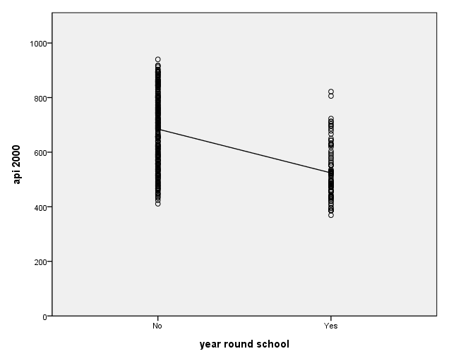
We can graph the observed values and the predicted values using the ggraph command as shown below. Although yr_rnd only has 2 values, we can still draw a regression line showing the relationship between yr_rnd and api00. Based on the results above, we see that the predicted value for non-year round schools is 684.539 and the predicted value for the year round schools is 524.032, and the slope of the line is negative, which makes sense since the coefficient for yr_rnd was negative (-160.5064). Note that the "type = scale" option is needed here because yr_rnd is an ordinal variable in the dataset.
GGRAPH
  /GRAPHDATASET NAME="GraphDataset" VARIABLES= api00 yr_rnd
  /GRAPHSPEC SOURCE=INLINE .
BEGIN GPL
SOURCE: s=userSource( id( "GraphDataset" ) )
DATA: yr_rnd=col(source(s), name("yr_rnd"), unit.category())
DATA: api00=col(source(s), name("api00"))
GUIDE: axis(dim(1), label("year round school"))
GUIDE: axis(dim(2), label("api 2000"))
SCALE: cat(dim(1), include("0", "1"))
SCALE: linear(dim(2), include(0))
ELEMENT: point(position(yr_rnd*api00))
ELEMENT: line( position(smooth.linear( yr_rnd * api00 ) ) )
END GPL.
Let's compare these predicted values to the mean api00 scores for the year-round and non-year-round students.
MEANS
  TABLES=api00 BY yr_rnd.
| Cases | ||||||
|---|---|---|---|---|---|---|
| Included | Excluded | Total | ||||
| N | Percent | N | Percent | N | Percent | |
| api 2000 * year round school | 400 | 100.0% | 0 | .0% | 400 | 100.0% |
| year round school | Mean | N | Std. Deviation |
|---|---|---|---|
| No | 684.54 | 308 | 132.113 |
| Yes | 524.03 | 92 | 98.916 |
| Total | 647.62 | 400 | 142.249 |
As you see, the regression equation predicts that the value of api00 will be the mean value of your group, depending on whether you went to year round school or non-year round school.
Let's relate these predicted values back to the regression equation. For the non-year-round students, their mean is the same as the intercept (684.539). The coefficient for yr_rnd is the amount we need to add to get the mean for the year-round students, i.e., we need to add -160.5064 to get 524.0326, the mean for the non year-round students. In other words, Byr_rnd is the mean api00 score for the year-round students minus the mean api00 score for the non year-round students, i.e., mean(year-round) - mean(non year-round).
It may be surprising to note that this regression analysis with a single dummy variable is the same as doing a t-test comparing the mean api00 for the year-round students with the non year-round students (see below). You can see that the t-value below is the same as the t-value for yr_rnd in the regression above. This is because Byr_rnd compares the non year-rounds and non year-rounds (since the coefficient is mean(year round)-mean(non year-round)).
T-TEST
  GROUPS=yr_rnd(0 1)
  /VARIABLES=api00.
| year round school | N | Mean | Std. Deviation | Std. Error Mean | |
|---|---|---|---|---|---|
| api 2000 | No | 308 | 684.54 | 132.113 | 7.528 |
| Yes | 92 | 524.03 | 98.916 | 10.313 |
| Levene's Test for Equality of Variances | t-test for Equality of Means | |||||||||
|---|---|---|---|---|---|---|---|---|---|---|
| F | Sig. | t | df | Sig. (2-tailed) | Mean Difference | Std. Error Difference | 95% Confidence Interval of the Difference | |||
| Lower | Upper | |||||||||
| api 2000 | Equal variances assumed | 20.539 | .000 | 10.782 | 398 | .000 | 160.51 | 14.887 | 131.239 | 189.774 |
| Equal variances not assumed | 12.571 | 197.215 | .000 | 160.51 | 12.768 | 135.327 | 185.686 | |||
Since a t-test is the same as doing an ANOVA, we can get the same results using the anova command as well. Note that in SPSS, when you click on "analyze" and "compare means," you can select a one-way ANOVA test. The code for conducting a one-way ANOVA is shown below. After this analysis, however, we will use the glm (for general linear model) command instead of the oneway command.
ONEWAY
  api00 BY yr_rnd.
| Sum of Squares | df | Mean Square | F | Sig. | |
|---|---|---|---|---|---|
| Between Groups | 1825000.563 | 1 | 1825000.563 | 116.241 | .000 |
| Within Groups | 6248671.435 | 398 | 15700.179 | ||
| Total | 8073671.998 | 399 |
Remember that if you square the t-value, you will get the F-value: 10.7815**2 = 116.24074 , showing another way in which the t-test is the same as the ANOVA test.
3.2 Regression with a 1/2 variable
A categorical predictor variable does not have to be coded 0/1 to be used in a regression model. It is easier to understand and interpret the results from a model with dummy variables, but the results from a variable coded 1/2 yield essentially the same results.
Let's make a copy of the variable yr_rnd called yr_rnd2 that is coded 1/2, 1=non year-round and 2=year-round.
compute yr_rnd2 = yr_rnd.
recode yr_rnd2 (0=1) (1=2).
execute.

REGRESSION
  /DEPENDENT api00
  /METHOD=ENTER yr_rnd2.
<some output omitted to save space>
Coefficients(a) Unstandardized Coefficients Standardized Coefficients t Sig. Model B Std. Error Beta
1 (Constant) 845.045 19.353 43.664 .000 YR_RND2 -160.506 14.887 -.475 -10.782 .000 a Dependent Variable: api 2000
Note that the coefficient for yr_rnd is the same as yr_rnd2. So, you can see that if you code yr_rnd as 0/1 or as 1/2, the regression coefficient works out to be the same. However the intercept is a bit less intuitive. When we used yr_rnd, the intercept was the mean for the non year-rounds. When using yr_rnd2, the intercept is the mean for the non year-rounds minus Byr_rnd2, i.e., 684.539 - (-160.506) = 845.045
Note that you can use 0/1 or 1/2 coding and the results for the coefficient come out the same, but the interpretation of constant in the regression equation is different. It is often easier to interpret the estimates for 0/1 coding.
In summary, these results indicate that the api00 scores are significantly different for the students depending on the type of school they attend, year round school vs. non-year round school. Those who attend non-year round school have significantly higher scores. Based on the regression results, those who attend non-year round schools have scores that are 160.5 points higher than those who attend year-round schools.
3.3 Regression with a 1/2/3 variable
3.3.1 Manually Creating Dummy Variables
Say that we would like to examine the relationship between the amount of poverty and
api scores. We don't have a measure of poverty, but we can use mealcat as
a proxy for a measure of poverty. You might be tempted to try including mealcat in a regression like this.
This is looking at the linear effect of mealcat with api00,
but mealcat is not an interval variable. Instead, you will want to code the variable so
that all the information concerning the three levels is accounted for.
You can dummy code mealcat like this.
We now have created mealcat1 that is 1 if mealcat is
1, and 0 otherwise. Likewise, mealcat2 is 1 if mealcat
is 2, and 0 otherwise; and likewise mealcat3 was created. We can see this
below.
We can now use two of these dummy variables (mealcat2 and mealcat3)
in the regression analysis.
regression
 /dependent api00
 /method=enter mealcat.
Model
Variables Entered
Variables Removed
Method
1
Percentage free meals in 3 categories(a)
.
Enter
a All requested variables entered. b Dependent Variable: api 2000
Model Summary
Model
R
R Square
Adjusted R Square
Std. Error of the Estimate
1
.867(a)
.752
.752
70.908
a Predictors: (Constant), Percentage free meals in 3 categories
Model
Sum of Squares
df
Mean Square
F
Sig.
1
Regression
6072527.519
1
6072527.519
1207.742
.000(a)
Residual
2001144.479
398
5028.001
Total
8073671.997
399
a Predictors: (Constant), Percentage free meals in 3 categories b Dependent Variable: api 2000
Coefficients(a)
Unstandardized Coefficients
Standardized Coefficients
t
Sig.
Model
B
Std. Error
Beta
1
(Constant)
950.987
9.422
100.935
.000
Percentage free meals in 3 categories
-150.553
4.332
-.867
-34.753
.000
a Dependent Variable: api 2000
if mealcat ~= missing(mealcat) mealcat1 = 0.
if mealcat = 1 mealcat1 = 1.
if mealcat ~= missing(mealcat) mealcat2 = 0.
if mealcat = 2 mealcat2 = 1.
if mealcat ~= missing(mealcat) mealcat3 = 0.
if mealcat = 3 mealcat3 = 1.
execute.
list mealcat mealcat1 mealcat2 mealcat3
 /cases from 1 to 10.

           MEALCAT MEALCAT1 MEALCAT2 MEALCAT3

                 2      .00     1.00      .00
                 3      .00      .00     1.00
                 3      .00      .00     1.00
                 3      .00      .00     1.00
                 3      .00      .00     1.00
                 1     1.00      .00      .00
                 1     1.00      .00      .00
                 1     1.00      .00      .00
                 1     1.00      .00      .00
                 1     1.00      .00      .00

Number of cases read:  10    Number of cases listed:  10
regression
 /dependent api00
 /method = enter mealcat2 mealcat3.
| Model | Variables Entered | Variables Removed | Method |
|---|---|---|---|
| 1 | MEALCAT3, MEALCAT2(a) | . | Enter |
| a All requested variables entered. | |||
| b Dependent Variable: api 2000 | |||
| Model | R | R Square | Adjusted R Square | Std. Error of the Estimate |
|---|---|---|---|---|
| 1 | .869(a) | .755 | .754 | 70.612 |
| a Predictors: (Constant), MEALCAT3, MEALCAT2 | ||||
| Model | Sum of Squares | df | Mean Square | F | Sig. | |
|---|---|---|---|---|---|---|
| 1 | Regression | 6094197.670 | 2 | 3047098.835 | 611.121 | .000(a) |
| Residual | 1979474.328 | 397 | 4986.081 | |||
| Total | 8073671.997 | 399 | ||||
| a Predictors: (Constant), MEALCAT3, MEALCAT2 | ||||||
| b Dependent Variable: api 2000 | ||||||
| Unstandardized Coefficients | Standardized Coefficients | t | Sig. | |||
|---|---|---|---|---|---|---|
| Model | B | Std. Error | Beta | |||
| 1 | (Constant) | 805.718 | 6.169 | 130.599 | .000 | |
| MEALCAT2 | -166.324 | 8.708 | -.550 | -19.099 | .000 | |
| MEALCAT3 | -301.338 | 8.629 | -1.007 | -34.922 | .000 | |
| a Dependent Variable: api 2000 | ||||||
We can test the overall differences among the three groups by using the /method = test statement as shown below. This shows that the overall differences among the three groups are significant, with an F value of 611.121 and a p value of .000.
regression
 /dependent api00
 /method = test (mealcat2 mealcat3).
| Model | Variables Entered | Variables Removed | Method |
|---|---|---|---|
| 1 | MEALCAT3, MEALCAT2 | . | Test |
| a Dependent Variable: api 2000 | |||
| Model | R | R Square | Adjusted R Square | Std. Error of the Estimate |
|---|---|---|---|---|
| 1 | .869(a) | .755 | .754 | 70.612 |
| a Predictors: (Constant), MEALCAT3, MEALCAT2 | ||||
| Model | Sum of Squares | df | Mean Square | F | Sig. | R Square Change | ||
|---|---|---|---|---|---|---|---|---|
| 1 | Subset Tests | MEALCAT2, MEALCAT3 | 6094197.670 | 2 | 3047098.835 | 611.121 | .000(a) | .755 |
| Regression | 6094197.670 | 2 | 3047098.835 | 611.121 | .000(b) | |||
| Residual | 1979474.328 | 397 | 4986.081 | |||||
| Total | 8073671.997 | 399 | ||||||
| a Tested against the full model. | ||||||||
| b Predictors in the Full Model: (Constant), MEALCAT3, MEALCAT2. | ||||||||
| c Dependent Variable: api 2000 | ||||||||
| Unstandardized Coefficients | Standardized Coefficients | t | Sig. | |||
|---|---|---|---|---|---|---|
| Model | B | Std. Error | Beta | |||
| 1 | (Constant) | 805.718 | 6.169 | 130.599 | .000 | |
| MEALCAT2 | -166.324 | 8.708 | -.550 | -19.099 | .000 | |
| MEALCAT3 | -301.338 | 8.629 | -1.007 | -34.922 | .000 | |
| a Dependent Variable: api 2000 | ||||||
The interpretation of the coefficients is much like that for the binary variables. Group 1 is the omitted group, so the constant is the mean for group 1. The coefficient for mealcat2 is the mean for group 2 minus the mean of the omitted group (group 1), and the coefficient for mealcat3 is the mean of group 3 minus the mean of group 1. You can verify this by comparing the coefficients with the means of the groups, shown below.
MEANS
  TABLES=api00 BY mealcat.
| Cases | ||||||
|---|---|---|---|---|---|---|
| Included | Excluded | Total | ||||
| N | Percent | N | Percent | N | Percent | |
| api 2000 * Percentage free meals in 3 categories | 400 | 100.0% | 0 | .0% | 400 | 100.0% |
| Percentage free meals in 3 categories | Mean | N | Std. Deviation |
|---|---|---|---|
| 0-46% free meals | 805.72 | 131 | 65.669 |
| 47-80% free meals | 639.39 | 132 | 82.135 |
| 81-100% free meals | 504.38 | 137 | 62.727 |
| Total | 647.62 | 400 | 142.249 |
Based on these results, we can say that the three groups differ in their api00 scores, and that in particular group2 is significantly different from group1 (because mealcat2 was significant) and group 3 is significantly different from group 1 (because mealcat3 was significant).
3.3.2 Using Do Loops
We can use the do repeat command to do the work for us to create the indicator (dummy) variables. This method is particularly useful when you need to create many indicator variables.
DO REPEAT A=mealcat1 mealcat2 mealcat3
 /B=1 2 3.
COMPUTE A=(mealcat=B).
END REPEAT.
We will then do a crosstab to verify that our indicator variables were created correctly.
crosstab /tables = mealcat by mealcat1
         /tables = mealcat by mealcat2
         /tables = mealcat by mealcat3.
Case Processing Summary Cases Valid Missing Total N Percent N Percent N Percent Percentage free meals in 3 categories * MEALCAT1 400 100.0% 0 .0% 400 100.0% Percentage free meals in 3 categories * MEALCAT2 400 100.0% 0 .0% 400 100.0% Percentage free meals in 3 categories * MEALCAT3 400 100.0% 0 .0% 400 100.0%
Percentage free meals in 3 categories * MEALCAT1 Crosstabulation
CountMEALCAT1 Total .00 1.00
Percentage free meals in 3 categories 0-46% free meals 131 131 47-80% free meals 132 132 81-100% free meals 137 137 Total 269 131 400
Percentage free meals in 3 categories * MEALCAT2 Crosstabulation
CountMEALCAT2 Total .00 1.00
Percentage free meals in 3 categories 0-46% free meals 131 131 47-80% free meals 132 132 81-100% free meals 137 137 Total 268 132 400
Percentage free meals in 3 categories * MEALCAT3 Crosstabulation
CountMEALCAT3 Total .00 1.00
Percentage free meals in 3 categories 0-46% free meals 131 131 47-80% free meals 132 132 81-100% free meals 137 137 Total 263 137 400
What if we wanted a different group to be the reference group? For example, let's omit group 3.
regression
 /dependent api00
 /method = enter mealcat1 mealcat2.
| Model | Variables Entered | Variables Removed | Method |
|---|---|---|---|
| 1 | MEALCAT2, MEALCAT1(a) | . | Enter |
| a All requested variables entered. | |||
| b Dependent Variable: api 2000 | |||
| Model | R | R Square | Adjusted R Square | Std. Error of the Estimate |
|---|---|---|---|---|
| 1 | .869(a) | .755 | .754 | 70.612 |
| a Predictors: (Constant), MEALCAT2, MEALCAT1 | ||||
| Model | Sum of Squares | df | Mean Square | F | Sig. | |
|---|---|---|---|---|---|---|
| 1 | Regression | 6094197.670 | 2 | 3047098.835 | 611.121 | .000(a) |
| Residual | 1979474.328 | 397 | 4986.081 | |||
| Total | 8073671.997 | 399 | ||||
| a Predictors: (Constant), MEALCAT2, MEALCAT1 | ||||||
| b Dependent Variable: api 2000 | ||||||
| Unstandardized Coefficients | Standardized Coefficients | t | Sig. | |||
|---|---|---|---|---|---|---|
| Model | B | Std. Error | Beta | |||
| 1 | (Constant) | 504.380 | 6.033 | 83.606 | .000 | |
| MEALCAT1 | 301.338 | 8.629 | .995 | 34.922 | .000 | |
| MEALCAT2 | 135.014 | 8.612 | .447 | 15.677 | .000 | |
| a Dependent Variable: api 2000 | ||||||
With group 3 omitted, the constant is now the mean of group 3 and mealcat1 is group1-group3 and mealcat2 is group2-group3. We see that both of these coefficients are significant, indicating that group 1 is significantly different from group 3 and group 2 is significantly different from group 3.
3.3.3 Using the glm command
We can also do this analysis using the glm command. The benefit of
the glm command is that it we don't need to manually create dummy
varaibles, and it gives us the test of the overall effect of mealcat
without needing to subsequently use the /method = test statement as we did with the regress
command.
We can use the /print=parameter statement with the glm
command to obtain the parameter estimates. Note that the estimates are
based on dummy coding with the last (third) category omitted, and correspond to
the results shown above where the third category was omitted. Note that the parameter estimates are the same because mealcat is coded
the same way in the regress command and in the glm command, because in both cases the last category (category 3) is being dropped. 3.3.4 Other coding schemes It is generally very convenient to use dummy coding, but that is not the only kind of
coding that can be used. As you have seen, when you use dummy coding one of the groups
becomes the reference group and all of the other groups are compared to that group. This
may not be the most interesting set of comparisons. Below is a list of the
types of coding schemes that SPSS will create for you. You can access
these through the pull-down menus, or you can request it on the /CONTRAST
statement when using GLM (described later). First, we show you how to
manually create the codes. Deviation(refcat): The deviations from the grand mean. Let's create a variable that compares group 1 with 2 and another variable that compares
group 2 with 3, and include those variables in the regression model. In
other words, we wish to create coefficients are comparisons of successive groups with group 1
as the baseline comparison group (i.e., the first comparison comparing group 1 vs. 2, and
the second comparison comparing groups 2 vs. 3). Below we show how to
manually generate
a coding scheme that forms these 2 comparisons.
We can perform this same series of comparisions much easier using the glm command with the contrast statement.
3.4 Regression with two categorical predictors Previously we looked at using yr_rnd to predict api00
And we have also looked at mealcat using the regression command
We can include both yr_rnd and mealcat together in the same model.
We can test the overall effect of mealcat with the method=test() command, which
is significant.
Because this model has only main effects (no interactions) you can interpret Byr_rnd
as the difference between the year round and non-year round group. The
coefficient for mealcat1 (which we will call Bmealcat1) is the difference between mealcat=1 and mealcat=3, and Bmealcat2 as
the difference between mealcat=2 and mealcat=3. Let's dig below the surface and see how the coefficients relate to the predicted
values. Let's view the cells formed by crossing yr_rnd and mealcat
and number the cells from cell1 to cell6. With respect to mealcat, the group mealcat=3 is the
reference category, and with respect to yr_rnd the group yr_rnd=0
is the reference category. As a result, cell3 is the reference cell. The constant is the
predicted value for this cell. The coefficient for yr_rnd is the difference between cell3
and cell6. Since this model has only main effects, it is also the
difference between cell2 and cell5, or from cell1 and cell4. In other words, Byr_rnd
is the amount you add to the predicted value when you go from non-year round to year round
schools. The coefficient for _Imealcat_1 is the predicted difference between
cell1 and cell3. Since this model only has main effects, it is also the predicted
difference between cell4 and cell6. Likewise, B_Imealcat_2 is the
predicted difference between cell2 and cell3, and also the predicted difference between
cell5 and cell6. So, the predicted values, in terms of the coefficients, would be We should note that if you computed the predicted values for each cell, they would not
exactly match the means in the 6 cells. The predicted means would be close to the
observed means in the cells, but not exactly the same. This is because our model
only has main effects and assumes that the difference between cell1 and cell4 is exactly
the same as the difference between cells 2 and 5 which is the same as the difference
between cells 3 and 5. Since the observed values don't follow this pattern, there is
some discrepancy between the predicted means and observed means.
3.4.2 Using the glm command We can run the same analysis using the glm command with just main
effects. Because SPSS's default is to include all main effects and
interactions in the model, to get just the main effects, you need to include the
/design statement and specify just the main effects, as shown
below.
glm
 api00 by mealcat.
Value Label
N
Percentage free meals in 3 categories
1
0-46% free meals
131
2
47-80% free meals
132
3
81-100% free meals
137
Tests of Between-Subjects Effects
Dependent Variable: api 2000
Source
Type III Sum of Squares
df
Mean Square
F
Sig.
Corrected Model
6094197.670(a)
2
3047098.835
611.121
.000
Intercept
168847142.059
1
168847142.059
33863.695
.000
MEALCAT
6094197.670
2
3047098.835
611.121
.000
Error
1979474.328
397
4986.081
Total
175839633.000
400
Corrected Total
8073671.997
399
a R Squared = .755 (Adjusted R Squared = .754)
glm
 api00 by mealcat
 /print=parameter.
Value Label
N
Percentage free meals in 3 categories
1
0-46% free meals
131
2
47-80% free meals
132
3
81-100% free meals
137
Tests of Between-Subjects Effects
Dependent Variable: api 2000
Source
Type III Sum of Squares
df
Mean Square
F
Sig.
Corrected Model
6094197.670(a)
2
3047098.835
611.121
.000
Intercept
168847142.059
1
168847142.059
33863.695
.000
MEALCAT
6094197.670
2
3047098.835
611.121
.000
Error
1979474.328
397
4986.081
Total
175839633.000
400
Corrected Total
8073671.997
399
a R Squared = .755 (Adjusted R Squared = .754)
Parameter Estimates
Dependent Variable: api 2000
B
Std. Error
t
Sig.
95% Confidence Interval
Parameter
Lower Bound
Upper Bound
Intercept
504.380
6.033
83.606
.000
492.519
516.240
[MEALCAT=1]
301.338
8.629
34.922
.000
284.374
318.302
[MEALCAT=2]
135.014
8.612
15.677
.000
118.083
151.945
[MEALCAT=3]
0(a)
.
.
.
.
.
a This parameter is set to zero because it is redundant.
Difference: The difference or reverse Helmert contrast - compare levels of a factor with the mean of the previous levels of the factor.
Simple(refcat): Compare each level of a factor to the last level.
Helmert: Compare levels of a factor with the mean of the subsequent levels of
the factor.
Polynomial: Orthogonal polynomial contrasts.
Repeated: Adjacent levels of a factor.
Special: A user-defined contrast.
if mealcat = 1 grp1 = .667.
if mealcat = 2 grp1 = -.333.
if mealcat = 3 grp1 = -.333.

if mealcat = 1 grp2 = .333.
if mealcat = 2 grp2 = .333.
if mealcat = 3 grp2 = -.667.
execute.

regression
 /dep = api00
 /method = enter grp1 grp2.
Model
Variables Entered
Variables Removed
Method
1
GRP2, GRP1(a)
.
Enter
a All requested variables entered. b Dependent Variable: api
2000
Model Summary
Model
R
R Square
Adjusted R Square
Std. Error of the Estimate
1
.869(a)
.755
.754
70.612
a Predictors: (Constant), GRP2, GRP1
Model
Sum of Squares
df
Mean Square
F
Sig.
1
Regression
6094197.670
2
3047098.835
611.121
.000(a)
Residual
1979474.328
397
4986.081
Total
8073671.997
399
a Predictors: (Constant), GRP2, GRP1 b Dependent Variable: api 2000
Coefficients(a)
Unstandardized Coefficients
Standardized Coefficients
t
Sig.
Model
B
Std. Error
Beta
1
(Constant)
649.820
3.531
184.016
.000
GRP1
166.324
8.708
.549
19.099
.000
GRP2
135.014
8.612
.451
15.677
.000
a Dependent Variable: api 2000
glm
 api00 by mealcat
 /contrast (mealcat)=repeated
 /print = parameter TEST(LMATRIX).
Value Label
N
Percentage free meals in 3 categories
1
0-46% free meals
131
2
47-80% free meals
132
3
81-100% free meals
137
Tests of Between-Subjects Effects
Dependent Variable: api 2000
Source
Type III Sum of Squares
df
Mean Square
F
Sig.
Corrected Model
6094197.670(a)
2
3047098.835
611.121
.000
Intercept
168847142.059
1
168847142.059
33863.695
.000
MEALCAT
6094197.670
2
3047098.835
611.121
.000
Error
1979474.328
397
4986.081
Total
175839633.000
400
Corrected Total
8073671.997
399
a R Squared = .755 (Adjusted R Squared = .754)
Parameter Estimates
Dependent Variable: api 2000
B
Std. Error
t
Sig.
95% Confidence Interval
Parameter
Lower Bound
Upper Bound
Intercept
504.380
6.033
83.606
.000
492.519
516.240
[MEALCAT=1]
301.338
8.629
34.922
.000
284.374
318.302
[MEALCAT=2]
135.014
8.612
15.677
.000
118.083
151.945
[MEALCAT=3]
0(a)
.
.
.
.
.
a This parameter is set to zero because it is redundant.
Intercept
Contrast
Parameter
L1
Intercept
1.000
[MEALCAT=1]
.333
[MEALCAT=2]
.333
[MEALCAT=3]
.333
The default display of this matrix is the transpose of the corresponding L matrix.
Based on Type III Sums of Squares.
MEALCAT
Contrast
Parameter
L2
L3
Intercept
0
0
[MEALCAT=1]
1
0
[MEALCAT=2]
0
1
[MEALCAT=3]
-1
-1
The default display of this matrix is the transpose of the corresponding L matrix.
Based on Type III Sums of Squares.
Contrast Coefficients (L' Matrix)
Percentage free meals in 3 categories Repeated Contrast
Parameter
Level 1 vs. Level 2
Level 2 vs. Level 3
Intercept
0
0
[MEALCAT=1]
1
0
[MEALCAT=2]
-1
1
[MEALCAT=3]
0
-1
The default display of this matrix is the transpose of the corresponding L matrix.
Contrast Results (K Matrix)
Dependent Variable
Percentage free meals in 3 categories Repeated Contrast
api 2000
Level 1 vs. Level 2
Contrast Estimate
166.324
Hypothesized Value
0
Difference (Estimate - Hypothesized)
166.324
Std. Error
8.708
Sig.
.000
95% Confidence Interval for Difference
Lower Bound
149.203
Upper Bound
183.444
Level 2 vs. Level 3
Contrast Estimate
135.014
Hypothesized Value
0
Difference (Estimate - Hypothesized)
135.014
Std. Error
8.612
Sig.
.000
95% Confidence Interval for Difference
Lower Bound
118.083
Upper Bound
151.945
Test Results
Dependent Variable: api 2000
Source
Sum of Squares
df
Mean Square
F
Sig.
Contrast
6094197.670
2
3047098.835
611.121
.000
Error
1979474.328
397
4986.081
If you compare the parameter estimates with the means you can verify that B1
(i.e., 0-46% free meals) is the mean of group 1 minus group 2, and B2
(i.e., 47-80% free meals) is the mean of group 2 minus group 3. Both of these
comparisons are significant, indicating that group 1 significantly differs from group 2,
and group 2 significantly differs from group 3.
MEANS
  TABLES=api00 BY mealcat.
Cases
Included
Excluded
Total
N
Percent
N
Percent
N
Percent
api 2000 * Percentage free meals in 3 categories
400
100.0%
0
.0%
400
100.0%
Report
api 2000
Percentage free meals in 3 categories
Mean
N
Std. Deviation
0-46% free meals
805.72
131
65.669
47-80% free meals
639.39
132
82.135
81-100% free meals
504.38
137
62.727
Total
647.62
400
142.249
regression
 /dep api00
 /method = enter yr_rnd.
Model
Variables Entered
Variables Removed
Method
1
year round school(a)
.
Enter
a All requested variables entered. b Dependent Variable: api 2000
Model Summary
Model
R
R Square
Adjusted R Square
Std. Error of the Estimate
1
.475(a)
.226
.224
125.300
a Predictors: (Constant), year round school
ANOVA(b)
Model
Sum of Squares
df
Mean Square
F
Sig.
1
Regression
1825000.563
1
1825000.563
116.241
.000(a)
Residual
6248671.435
398
15700.179
Total
8073671.997
399
a Predictors: (Constant), year round school b Dependent Variable: api 2000
Coefficients(a)
Unstandardized Coefficients
Standardized Coefficients
t
Sig.
Model
B
Std. Error
Beta
1
(Constant)
684.539
7.140
95.878
.000
year round school
-160.506
14.887
-.475
-10.782
.000
a Dependent Variable: api 2000
regression
 /dep api00
 /method =  enter mealcat1 mealcat2.
Model
Variables Entered
Variables Removed
Method
1
MEALCAT2, MEALCAT1(a)
.
Enter
a All requested variables entered. b Dependent Variable: api 2000
Model Summary
Model
R
R Square
Adjusted R Square
Std. Error of the Estimate
1
.869(a)
.755
.754
70.612
a Predictors: (Constant), MEALCAT2, MEALCAT1
ANOVA(b)
Model
Sum of Squares
df
Mean Square
F
Sig.
1
Regression
6094197.670
2
3047098.835
611.121
.000(a)
Residual
1979474.328
397
4986.081
Total
8073671.997
399
a Predictors: (Constant), MEALCAT2, MEALCAT1 b Dependent Variable: api 2000
Coefficients(a)
Unstandardized Coefficients
Standardized Coefficients
t
Sig.
Model
B
Std. Error
Beta
1
(Constant)
504.380
6.033
83.606
.000
MEALCAT1
301.338
8.629
.995
34.922
.000
MEALCAT2
135.014
8.612
.447
15.677
.000
a Dependent Variable: api 2000
regression
 /dep api00
 /method =  enter yr_rnd mealcat1 mealcat2.
Model
Variables Entered
Variables Removed
Method
1
MEALCAT2, year round school, MEALCAT1(a)
.
Enter
a All requested variables entered. b Dependent Variable: api 2000
Model Summary
Model
R
R Square
Adjusted R Square
Std. Error of the Estimate
1
.876(a)
.767
.765
68.893
a Predictors: (Constant), MEALCAT2, year round school, MEALCAT1
ANOVA(b)
Model
Sum of Squares
df
Mean Square
F
Sig.
1
Regression
6194144.303
3
2064714.768
435.017
.000(a)
Residual
1879527.694
396
4746.282
Total
8073671.997
399
a Predictors: (Constant), MEALCAT2, year round school, MEALCAT1 b Dependent Variable: api 2000
Coefficients(a)
Unstandardized Coefficients
Standardized Coefficients
t
Sig.
Model
B
Std. Error
Beta
1
(Constant)
526.330
7.585
69.395
.000
year round school
-42.960
9.362
-.127
-4.589
.000
MEALCAT1
281.683
9.446
.930
29.821
.000
MEALCAT2
117.946
9.189
.390
12.836
.000
a Dependent Variable: api 2000
regression
 /dep api00
 /method =  enter yr_rnd
 /method = test(mealcat1 mealcat2).
Model
Variables Entered
Variables Removed
Method
1
year round school(a)
.
Enter
2
MEALCAT2, MEALCAT1
.
Test
a All requested variables entered. b Dependent Variable: api 2000
Model Summary
Model
R
R Square
Adjusted R Square
Std. Error of the Estimate
1
.475(a)
.226
.224
125.300
2
.876(b)
.767
.765
68.893
a Predictors: (Constant), year round school b Predictors: (Constant), year round school, MEALCAT2, MEALCAT1
ANOVA(d)
Model
Sum of Squares
df
Mean Square
F
Sig.
R Square Change
1
Regression
1825000.563
1
1825000.563
116.241
.000(a)
Residual
6248671.435
398
15700.179
Total
8073671.997
399
2
Subset Tests
MEALCAT1, MEALCAT2
4369143.740
2
2184571.870
460.270
.000(b)
.541
Regression
6194144.303
3
2064714.768
435.017
.000(c)
Residual
1879527.694
396
4746.282
Total
8073671.997
399
a Predictors: (Constant), year round school b Tested against the full model. c Predictors in the Full Model: (Constant), year round school, MEALCAT2, MEALCAT1. d Dependent Variable: api 2000
Coefficients(a)
Unstandardized Coefficients
Standardized Coefficients
t
Sig.
Model
B
Std. Error
Beta
1
(Constant)
684.539
7.140
95.878
.000
year round school
-160.506
14.887
-.475
-10.782
.000
2
(Constant)
526.330
7.585
69.395
.000
year round school
-42.960
9.362
-.127
-4.589
.000
MEALCAT1
281.683
9.446
.930
29.821
.000
MEALCAT2
117.946
9.189
.390
12.836
.000
a Dependent Variable: api 2000
Excluded Variables(b)
Beta In
t
Sig.
Partial Correlation
Collinearity Statistics
Model
Tolerance
1
MEALCAT1
.697(a)
23.132
.000
.758
.914
MEALCAT2
-.138(a)
-3.106
.002
-.154
.962
a Predictors in the Model: (Constant), year round school b Dependent Variable: api 2000
           mealcat=1     mealcat=2      mealcat=3
 yr_rnd=0  cell1         cell2          cell3
 yr_rnd=1  cell4         cell5          cell6
           mealcat=1         mealcat=2         mealcat=3
          -----------------------------------------------
 yr_rnd=0  intercept         intercept        intercept
           +BMealCat1       +BMealCat2
          -----------------------------------------------
 yr_rnd=1  intercept        intercept         intercept
           +Byr_rnd          +Byr_rnd          +Byr_rnd
           +BMealCat1       +BMealCat2
glm
  api00 BY yr_rnd mealcat
  /DESIGN = yr_rnd mealcat
  /print=parameter TEST(LMATRIX).
Value Label
N
year round school
0
No
308
1
Yes
92
Percentage free meals in 3 categories
1
0-46% free meals
131
2
47-80% free meals
132
3
81-100% free meals
137
| Source | Type III Sum of Squares | df | Mean Square | F | Sig. |
|---|---|---|---|---|---|
| Corrected Model | 6194144.303(a) | 3 | 2064714.768 | 435.017 | .000 |
| Intercept | 104733334.071 | 1 | 104733334.071 | 22066.395 | .000 |
| YR_RND | 99946.633 | 1 | 99946.633 | 21.058 | .000 |
| MEALCAT | 4369143.740 | 2 | 2184571.870 | 460.270 | .000 |
| Error | 1879527.694 | 396 | 4746.282 | ||
| Total | 175839633.000 | 400 | |||
| Corrected Total | 8073671.997 | 399 | |||
| a R Squared = .767 (Adjusted R Squared = .765) | |||||
| B | Std. Error | t | Sig. | 95% Confidence Interval | ||
|---|---|---|---|---|---|---|
| Parameter | Lower Bound | Upper Bound | ||||
| Intercept | 483.370 | 7.457 | 64.821 | .000 | 468.710 | 498.030 |
| [YR_RND=0] | 42.960 | 9.362 | 4.589 | .000 | 24.555 | 61.365 |
| [YR_RND=1] | 0(a) | . | . | . | . | . |
| [MEALCAT=1] | 281.683 | 9.446 | 29.821 | .000 | 263.113 | 300.253 |
| [MEALCAT=2] | 117.946 | 9.189 | 12.836 | .000 | 99.881 | 136.011 |
| [MEALCAT=3] | 0(a) | . | . | . | . | . |
| a This parameter is set to zero because it is redundant. | ||||||
| Contrast | |
|---|---|
| Parameter | L1 |
| Intercept | 1.000 |
| [YR_RND=0] | .500 |
| [YR_RND=1] | .500 |
| [MEALCAT=1] | .333 |
| [MEALCAT=2] | .333 |
| [MEALCAT=3] | .333 |
| The default display of this matrix is the transpose of the corresponding L matrix. Based on Type III Sums of Squares. | |
| Contrast | |
|---|---|
| Parameter | L2 |
| Intercept | 0 |
| [YR_RND=0] | 1 |
| [YR_RND=1] | -1 |
| [MEALCAT=1] | 0 |
| [MEALCAT=2] | 0 |
| [MEALCAT=3] | 0 |
| The default display of this matrix is the transpose of the corresponding L matrix. Based on Type III Sums of Squares. | |
| Contrast | ||
|---|---|---|
| Parameter | L4 | L5 |
| Intercept | 0 | 0 |
| [YR_RND=0] | 0 | 0 |
| [YR_RND=1] | 0 | 0 |
| [MEALCAT=1] | 1 | 0 |
| [MEALCAT=2] | 0 | 1 |
| [MEALCAT=3] | -1 | -1 |
| The default display of this matrix is the transpose of the corresponding L matrix. Based on Type III Sums of Squares. | ||
In summary, these results indicate the differences between year round and non-year
round students is significant, and the differences among the three mealcat
groups are significant.
3.5 Categorical predictor with interactions
3.5.1 Manually coding an interaction
Let's perform the same analysis that we performed above. This time let's include the interaction of mealcat by yr_rnd.
compute yrmeal1 = mealcat1*yr_rnd.
compute yrmeal2 = mealcat2*yr_rnd.
execute.

regression
 /dep api00
 /method = enter yr_rnd mealcat1 mealcat2 yrmeal1 yrmeal2.
| Model | Variables Entered | Variables Removed | Method |
|---|---|---|---|
| 1 | YRMEAL2, YRMEAL1, MEALCAT1, year round school, MEALCAT2(a) | . | Enter |
| a All requested variables entered. | |||
| b Dependent Variable: api 2000 | |||
| Model | R | R Square | Adjusted R Square | Std. Error of the Estimate |
|---|---|---|---|---|
| 1 | .877(a) | .769 | .766 | 68.873 |
| a Predictors: (Constant), YRMEAL2, YRMEAL1, MEALCAT1, year round school, MEALCAT2 | ||||
| Model | Sum of Squares | df | Mean Square | F | Sig. | |
|---|---|---|---|---|---|---|
| 1 | Regression | 6204727.822 | 5 | 1240945.564 | 261.609 | .000(a) |
| Residual | 1868944.176 | 394 | 4743.513 | |||
| Total | 8073671.997 | 399 | ||||
| a Predictors: (Constant), YRMEAL2, YRMEAL1, MEALCAT1, year round school, MEALCAT2 | ||||||
| b Dependent Variable: api 2000 | ||||||
| Unstandardized Coefficients | Standardized Coefficients | t | Sig. | |||
|---|---|---|---|---|---|---|
| Model | B | Std. Error | Beta | |||
| 1 | (Constant) | 521.493 | 8.414 | 61.978 | .000 | |
| year round school | -33.493 | 11.771 | -.099 | -2.845 | .005 | |
| MEALCAT1 | 288.193 | 10.443 | .952 | 27.597 | .000 | |
| MEALCAT2 | 123.781 | 10.552 | .410 | 11.731 | .000 | |
| YRMEAL1 | -40.764 | 29.231 | -.038 | -1.395 | .164 | |
| YRMEAL2 | -18.248 | 22.256 | -.024 | -.820 | .413 | |
| a Dependent Variable: api 2000 | ||||||
We can test the overall interaction with the test command. This interaction effect is not significant, with an F of 1.116 and a p value of .329.
regression
 /dep api00
 /method = enter yr_rnd mealcat1 mealcat2
 /method = test(yrmeal1 yrmeal2).
| Model | Variables Entered | Variables Removed | Method |
|---|---|---|---|
| 1 | MEALCAT2, year round school, MEALCAT1(a) | . | Enter |
| 2 | YRMEAL1, YRMEAL2 | . | Test |
| a All requested variables entered. | |||
| b Dependent Variable: api 2000 | |||
| Model | R | R Square | Adjusted R Square | Std. Error of the Estimate |
|---|---|---|---|---|
| 1 | .876(a) | .767 | .765 | 68.893 |
| 2 | .877(b) | .769 | .766 | 68.873 |
| a Predictors: (Constant), MEALCAT2, year round school, MEALCAT1 | ||||
| b Predictors: (Constant), MEALCAT2, year round school, MEALCAT1, YRMEAL1, YRMEAL2 | ||||
| Model | Sum of Squares | df | Mean Square | F | Sig. | R Square Change | ||
|---|---|---|---|---|---|---|---|---|
| 1 | Regression | 6194144.303 | 3 | 2064714.768 | 435.017 | .000(a) | ||
| Residual | 1879527.694 | 396 | 4746.282 | |||||
| Total | 8073671.997 | 399 | ||||||
| 2 | Subset Tests | YRMEAL1, YRMEAL2 | 10583.519 | 2 | 5291.759 | 1.116 | .329(b) | .001 |
| Regression | 6204727.822 | 5 | 1240945.564 | 261.609 | .000(c) | |||
| Residual | 1868944.176 | 394 | 4743.513 | |||||
| Total | 8073671.997 | 399 | ||||||
| a Predictors: (Constant), MEALCAT2, year round school, MEALCAT1 | ||||||||
| b Tested against the full model. | ||||||||
| c Predictors in the Full Model: (Constant), MEALCAT2, year round school, MEALCAT1, YRMEAL1, YRMEAL2. | ||||||||
| d Dependent Variable: api 2000 | ||||||||
| Unstandardized Coefficients | Standardized Coefficients | t | Sig. | |||
|---|---|---|---|---|---|---|
| Model | B | Std. Error | Beta | |||
| 1 | (Constant) | 526.330 | 7.585 | 69.395 | .000 | |
| year round school | -42.960 | 9.362 | -.127 | -4.589 | .000 | |
| MEALCAT1 | 281.683 | 9.446 | .930 | 29.821 | .000 | |
| MEALCAT2 | 117.946 | 9.189 | .390 | 12.836 | .000 | |
| 2 | (Constant) | 521.493 | 8.414 | 61.978 | .000 | |
| year round school | -33.493 | 11.771 | -.099 | -2.845 | .005 | |
| MEALCAT1 | 288.193 | 10.443 | .952 | 27.597 | .000 | |
| MEALCAT2 | 123.781 | 10.552 | .410 | 11.731 | .000 | |
| YRMEAL1 | -40.764 | 29.231 | -.038 | -1.395 | .164 | |
| YRMEAL2 | -18.248 | 22.256 | -.024 | -.820 | .413 | |
| a Dependent Variable: api 2000 | ||||||
| Beta In | t | Sig. | Partial Correlation | Collinearity Statistics | ||
|---|---|---|---|---|---|---|
| Model | Tolerance | |||||
| 1 | YRMEAL1 | -.033(a) | -1.249 | .212 | -.063 | .846 |
| YRMEAL2 | -.016(a) | -.535 | .593 | -.027 | .695 | |
| a Predictors in the Model: (Constant), MEALCAT2, year round school, MEALCAT1 | ||||||
| b Dependent Variable: api 2000 | ||||||
It is important to note how the meaning of the coefficients change in the presence of these interaction terms. For example, in the prior model, with only main effects, we could interpret Byr_rnd as the difference between the year-round and non- year-round students. However, now that we have added the interaction term, the term Byr_rnd represents the difference between cell3 and cell6, or the difference between the year- round and non-year round students when mealcat=3 (because mealcat=3 was the omitted group). The presence of an interaction would imply that the difference between year round and non-year-round students depends on the level of mealcat. The interaction terms Byrmeal1 and Byrmeal2 represent the extent to which the difference between the year-round/non- year- round students changes when mealcat=1 and when mealcat=2 (as compared to the reference group, mealcat=3). For example, the term Byrmeal1 represents the difference between year- round and non-year- round for mealcat=1 vs. the difference for mealcat=3. In other words, Byrmeal1 in this design is (cell1-cell4) - (cell3-cell6), or it represents how much the effect of yr_rnd differs between mealcat=1 and mealcat=3.
Below we have shown the predicted values for the six cells in terms of the coefficients in the model. If you compare this to the main effects model, you will see that the predicted values are the same except for the addition of yrmeal1 (in cell 4) and yrmeal2 (in cell 5).
           mealcat=1           mealcat=2         mealcat=3
           -------------------------------------------------
 yr_rnd=0  intercept           intercept        intercept
           +BMealCat1         +BMealCat2
           -------------------------------------------------
 yr_rnd=1  intercept          intercept         intercept
           +Byr_rnd            +Byr_rnd          +Byr_rnd
           +BMealCat1         +BMealCat2
           +YrMeal1            +YrMeal2
It can be very tricky to interpret these interaction terms if you wish to form specific comparisons. For example, if you wanted to perform a test of the simple main effect of yr_rnd when mealcat=1, i.e., comparing compare cell1 with cell4, you would want to compare intercept+ BMealCat1 vs. intercept + Byr_rnd + BMealCat1 + BYrMeal1. As we will see, such tests can be more easily done via glm.
3.5.2 Using glm
Constructing these interactions can be somewhat easier when using the glm command. As you see below, the glm command gives us the test of the overall main effects and interactions without the need to perform subsequent test statement. The /emmeans statement tells SPSS to compare each level of the categorical variable with every other level of that variable.
glm
  api00 by yr_rnd mealcat
  /EMMEANS TABLES(yr_rnd*mealcat) COMPARE(yr_rnd).
| Value Label | N | ||
|---|---|---|---|
| year round school | 0 | No | 308 |
| 1 | Yes | 92 | |
| Percentage free meals in 3 categories | 1 | 0-46% free meals | 131 |
| 2 | 47-80% free meals | 132 | |
| 3 | 81-100% free meals | 137 | |
| Source | Type III Sum of Squares | df | Mean Square | F | Sig. |
|---|---|---|---|---|---|
| Corrected Model | 6204727.822(a) | 5 | 1240945.564 | 261.609 | .000 |
| Intercept | 56354756.653 | 1 | 56354756.653 | 11880.384 | .000 |
| YR_RND | 99617.371 | 1 | 99617.371 | 21.001 | .000 |
| MEALCAT | 1796232.798 | 2 | 898116.399 | 189.336 | .000 |
| YR_RND * MEALCAT | 10583.519 | 2 | 5291.759 | 1.116 | .329 |
| Error | 1868944.176 | 394 | 4743.513 | ||
| Total | 175839633.000 | 400 | |||
| Corrected Total | 8073671.997 | 399 | |||
| a R Squared = .769 (Adjusted R Squared = .766) | |||||
| Mean | Std. Error | 95% Confidence Interval | |||
|---|---|---|---|---|---|
| year round school | Percentage free meals in 3 categories | Lower Bound | Upper Bound | ||
| No | 0-46% free meals | 809.685 | 6.185 | 797.526 | 821.845 |
| 47-80% free meals | 645.274 | 6.367 | 632.755 | 657.792 | |
| 81-100% free meals | 521.493 | 8.414 | 504.950 | 538.035 | |
| Yes | 0-46% free meals | 735.429 | 26.032 | 684.250 | 786.607 |
| 47-80% free meals | 593.533 | 17.783 | 558.572 | 628.495 | |
| 81-100% free meals | 488.000 | 8.232 | 471.816 | 504.184 | |
| Mean Difference (I-J) | Std. Error | Sig.(a) | 95% Confidence Interval for Difference(a) | ||||
|---|---|---|---|---|---|---|---|
| Percentage free meals in 3 categories | (I) year round school | (J) year round school | Lower Bound | Upper Bound | |||
| 0-46% free meals | No | Yes | 74.257(*) | 26.756 | .006 | 21.654 | 126.860 |
| Yes | No | -74.257(*) | 26.756 | .006 | -126.860 | -21.654 | |
| 47-80% free meals | No | Yes | 51.740(*) | 18.889 | .006 | 14.605 | 88.875 |
| Yes | No | -51.740(*) | 18.889 | .006 | -88.875 | -14.605 | |
| 81-100% free meals | No | Yes | 33.493(*) | 11.771 | .005 | 10.350 | 56.635 |
| Yes | No | -33.493(*) | 11.771 | .005 | -56.635 | -10.350 | |
| Based on estimated marginal means | |||||||
| * The mean difference is significant at the .050 level. | |||||||
| a Adjustment for multiple comparisons: Least Significant Difference (equivalent to no adjustments). | |||||||
| Percentage free meals in 3 categories | Sum of Squares | df | Mean Square | F | Sig. | |
|---|---|---|---|---|---|---|
| 0-46% free meals | Contrast | 36536.101 | 1 | 36536.101 | 7.702 | .006 |
| Error | 1868944.176 | 394 | 4743.513 | |||
| 47-80% free meals | Contrast | 35592.534 | 1 | 35592.534 | 7.503 | .006 |
| Error | 1868944.176 | 394 | 4743.513 | |||
| 81-100% free meals | Contrast | 38401.517 | 1 | 38401.517 | 8.096 | .005 |
| Error | 1868944.176 | 394 | 4743.513 | |||
| Each F tests the simple effects of year round school within each level combination of the other effects shown. These tests are based on the linearly independent pairwise comparisons among the estimated marginal means. | ||||||
Although this section has focused on how to handle analyses involving interactions, these particular results show no indication of interaction. We could decide to omit interaction terms from future analyses having found the interactions to be non-significant. This would simplify future analyses, however including the interaction term can be useful to assure readers that the interaction term is non-significant.
3.6 Continuous and Categorical variables
3.6.1 Using regress
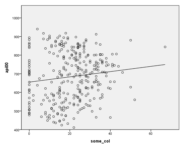
Say that we wish to analyze both continuous and categorical variables in one analysis. For example, let's include yr_rnd and some_col in the same analysis. We will save the predicted values for use in just a moment.
regress
 /dep = api00
 /method = enter yr_rnd some_col
 /save pre.
Variables Entered/Removed(b) Model Variables Entered Variables Removed Method 1 parent some college, year round school(a) . Enter a All requested variables entered. b Dependent Variable: api 2000
Model Summary(b)Model R R Square Adjusted R Square Std. Error of the Estimate 1 .507(a) .257 .253 122.951 a Predictors: (Constant), parent some college, year round school b Dependent Variable: api 2000
ANOVA(b) Model Sum of Squares df Mean Square F Sig. 1 Regression 2072201.839 2 1036100.919 68.539 .000(a) Residual 6001470.159 397 15117.053 Total 8073671.997 399 a Predictors: (Constant), parent some college, year round school b Dependent Variable: api 2000
Coefficients(a)Unstandardized Coefficients Standardized Coefficients t Sig. Model B Std. Error Beta
1 (Constant) 637.858 13.503 47.237 .000 year round school -149.159 14.875 -.442 -10.027 .000 parent some college 2.236 .553 .178 4.044 .000 a Dependent Variable: api 2000
Residuals Statistics(a)Minimum Maximum Mean Std. Deviation N Predicted Value 488.70 787.65 647.62 72.066 400 Residual -276.04 293.20 .00 122.643 400 Std. Predicted Value -2.205 1.943 .000 1.000 400 Std. Residual -2.245 2.385 .000 .997 400 a Dependent Variable: api 2000
Let's graph the predicted values by some_col.
GRAPH
  /SCATTERPLOT(BIVAR)=some_col WITH pre_1.
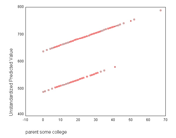
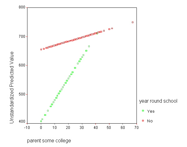
The coefficient for some_col indicates that for every unit increase in some_col the api00 score is predicted to increase by 2.23 units. This is the slope of the lines shown in the above graph. The graph has two lines, one for the year round students and one for the non-year round students. The coefficient for yr_rnd is -149.16, indicating that as yr_rnd increases by 1 unit, the api00 score is expected to decrease by about 149 units. As you can see in the graph, the top line is about 150 units higher than the lower line. You can see that the intercept is 637 and that is where the upper line crosses the Y axis when X is 0. The lower line crosses the line about 150 units lower at about 487.
3.6.2 Using glm
We can run this analysis using the glm command. The glm command assumes that the variables are categorical; thus, we need to enter some_col as a covariate to specify that some_col is a continuous variable.
glm
 api00 by yr_rnd with some_col.
| Value Label | N | ||
|---|---|---|---|
| year round school | 0 | No | 308 |
| 1 | Yes | 92 | |
| Source | Type III Sum of Squares | df | Mean Square | F | Sig. |
|---|---|---|---|---|---|
| Corrected Model | 2072201.839(a) | 2 | 1036100.919 | 68.539 | .000 |
| Intercept | 30709901.014 | 1 | 30709901.014 | 2031.474 | .000 |
| SOME_COL | 247201.276 | 1 | 247201.276 | 16.352 | .000 |
| YR_RND | 1519992.669 | 1 | 1519992.669 | 100.548 | .000 |
| Error | 6001470.159 | 397 | 15117.053 | ||
| Total | 175839633.000 | 400 | |||
| Corrected Total | 8073671.997 | 399 | |||
| a R Squared = .257 (Adjusted R Squared = .253) | |||||
If we square the t-values from the regress command (above), we would find that they match those of the glm command.
3.7 Interactions of Continuous by 0/1 Categorical variables
Above we showed an analysis that looked at the relationship between some_col and api00 and also included yr_rnd. We saw that this produced a graph where we saw the relationship between some_col and api00 but there were two regression lines, one higher than the other but with equal slopes. Such a model assumed that the slope was the same for the two groups. Perhaps the slope might be different for these groups. Let's run the regressions separately for these two groups beginning with the non-year-round schools.
COMPUTE filt=(yr_rnd=0).
FILTER BY filt.
regress
 /dep = api00
 /method = enter some_col.
| Model | Variables Entered | Variables Removed | Method |
|---|---|---|---|
| 1 | parent some college(a) | . | Enter |
| a All requested variables entered. | |||
| b Dependent Variable: api 2000 | |||
| Model | R | R Square | Adjusted R Square | Std. Error of the Estimate |
|---|---|---|---|---|
| 1 | .126(a) | .016 | .013 | 131.278 |
| a Predictors: (Constant), parent some college | ||||
| Model | Sum of Squares | df | Mean Square | F | Sig. | |
|---|---|---|---|---|---|---|
| 1 | Regression | 84700.858 | 1 | 84700.858 | 4.915 | .027(a) |
| Residual | 5273591.675 | 306 | 17233.960 | |||
| Total | 5358292.532 | 307 | ||||
| a Predictors: (Constant), parent some college | ||||||
| b Dependent Variable: api 2000 | ||||||
| Unstandardized Coefficients | Standardized Coefficients | t | Sig. | |||
|---|---|---|---|---|---|---|
| Model | B | Std. Error | Beta | |||
| 1 | (Constant) | 655.110 | 15.237 | 42.995 | .000 | |
| parent some college | 1.409 | .636 | .126 | 2.217 | .027 | |
| a Dependent Variable: api 2000 | ||||||
GGRAPH
  /GRAPHDATASET NAME="GraphDataset" VARIABLES= api00 some_col
  /GRAPHSPEC SOURCE=INLINE .
BEGIN GPL
SOURCE: s=userSource( id( "GraphDataset" ) )
DATA: api00=col( source(s), name( "api00" ) )
DATA: some_col=col( source(s), name( "some_col" ) )
GUIDE: axis( dim( 1 ), label( "some_col" ) )
GUIDE: axis( dim( 2 ), label( "api00" ) )
ELEMENT: point( position( some_col * api00 ) )
ELEMENT: line( position(smooth.linear( some_col * api00 ) ) )
END GPL.
COMMENT -- End GGRAPH command.
filter off.
Likewise, let's look at the year-round schools.
COMPUTE filt=(yr_rnd=1).
FILTER BY filt.
regress
 /dep = api00
 /method = enter some_col.
| Model | Variables Entered | Variables Removed | Method |
|---|---|---|---|
| 1 | parent some college(a) | . | Enter |
| a All requested variables entered. | |||
| b Dependent Variable: api 2000 | |||
| Model | R | R Square | Adjusted R Square | Std. Error of the Estimate |
|---|---|---|---|---|
| 1 | .648(a) | .420 | .413 | 75.773 |
| a Predictors: (Constant), parent some college | ||||
| Model | Sum of Squares | df | Mean Square | F | Sig. | |
|---|---|---|---|---|---|---|
| 1 | Regression | 373644.064 | 1 | 373644.064 | 65.078 | .000(a) |
| Residual | 516734.838 | 90 | 5741.498 | |||
| Total | 890378.902 | 91 | ||||
| a Predictors: (Constant), parent some college | ||||||
| b Dependent Variable: api 2000 | ||||||
| Unstandardized Coefficients | Standardized Coefficients | t | Sig. | |||
|---|---|---|---|---|---|---|
| Model | B | Std. Error | Beta | |||
| 1 | (Constant) | 407.039 | 16.515 | 24.647 | .000 | |
| parent some college | 7.403 | .918 | .648 | 8.067 | .000 | |
| a Dependent Variable: api 2000 | ||||||
GGRAPH
  /GRAPHDATASET NAME="GraphDataset" VARIABLES= api00 some_col
  /GRAPHSPEC SOURCE=INLINE .
BEGIN GPL
SOURCE: s=userSource( id( "GraphDataset" ) )
DATA: api00=col( source(s), name( "api00" ) )
DATA: some_col=col( source(s), name( "some_col" ) )
GUIDE: axis( dim( 1 ), label( "some_col" ) )
GUIDE: axis( dim( 2 ), label( "api00" ) )
ELEMENT: point( position( some_col * api00 ) )
ELEMENT: line( position(smooth.linear( some_col * api00 ) ) )
END GPL.
filter off.
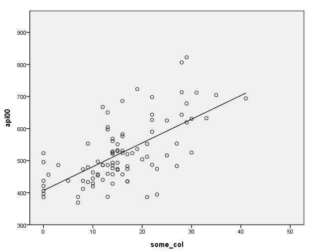
Note that the slope of the regression line looks much steeper for the year-round schools than for the non-year-round schools. This is confirmed by the regression equations that show the slope for the year round schools to be higher (7.4) than non-year round schools (1.3). We can compare these to see if these are significantly different from each other by including the interaction of some_col by yr_rnd, an interaction of a continuous variable by a categorical variable.
3.7.1 Computing interactions manually
We will start by manually computing the interaction of some_col by yr_rnd. Let's start fresh and reload the elemapi2 data file to clear out any variables we had previously created.
GET FILE='C:spssregelemapi2.sav'.
Next, let's make a variable that is the interaction of some college (some_col) and year-round schools (yr_rnd) called yrXsome.
compute yrXsome = yr_rnd*some_col.
execute.
We can now run the regression that tests whether the coefficient for some_col is significantly different for year round schools and non-year- round schools. Indeed, the yrXsome interaction effect is significant. We can make a graph showing the regression lines for the two types of schools showing how different their regression lines are, so we will save the predicted values.
regress
 /dep = api00
 /method = enter some_col yr_rnd yrXsome
 /save pre.
| Model | Variables Entered | Variables Removed | Method |
|---|---|---|---|
| 1 | YRXSOME, parent some college, year round school(a) | . | Enter |
| a All requested variables entered. | |||
| b Dependent Variable: api 2000 | |||
| Model | R | R Square | Adjusted R Square | Std. Error of the Estimate |
|---|---|---|---|---|
| 1 | .532(a) | .283 | .277 | 120.922 |
| a Predictors: (Constant), YRXSOME, parent some college, year round school | ||||
| b Dependent Variable: api 2000 | ||||
| Model | Sum of Squares | df | Mean Square | F | Sig. | |
|---|---|---|---|---|---|---|
| 1 | Regression | 2283345.485 | 3 | 761115.162 | 52.053 | .000(a) |
| Residual | 5790326.513 | 396 | 14622.037 | |||
| Total | 8073671.997 | 399 | ||||
| a Predictors: (Constant), YRXSOME, parent some college, year round school | ||||||
| b Dependent Variable: api 2000 | ||||||
| Unstandardized Coefficients | Standardized Coefficients | t | Sig. | |||
|---|---|---|---|---|---|---|
| Model | B | Std. Error | Beta | |||
| 1 | (Constant) | 655.110 | 14.035 | 46.677 | .000 | |
| parent some college | 1.409 | .586 | .112 | 2.407 | .017 | |
| year round school | -248.071 | 29.859 | -.735 | -8.308 | .000 | |
| YRXSOME | 5.993 | 1.577 | .330 | 3.800 | .000 | |
| a Dependent Variable: api 2000 | ||||||
| Minimum | Maximum | Mean | Std. Deviation | N | |
|---|---|---|---|---|---|
| Predicted Value | 407.04 | 749.54 | 647.62 | 75.648 | 400 |
| Residual | -275.12 | 279.25 | .00 | 120.466 | 400 |
| Std. Predicted Value | -3.180 | 1.347 | .000 | 1.000 | 400 |
| Std. Residual | -2.275 | 2.309 | .000 | .996 | 400 |
| a Dependent Variable: api 2000 | |||||
We can graph the predicted values for the two types of schools by some_col. You can see how the two lines have quite different slopes, consistent with the fact that the yrXsome interaction was significant.
GRAPH
  /SCATTERPLOT(BIVAR)=some_col WITH pre_1 BY yr_rnd.
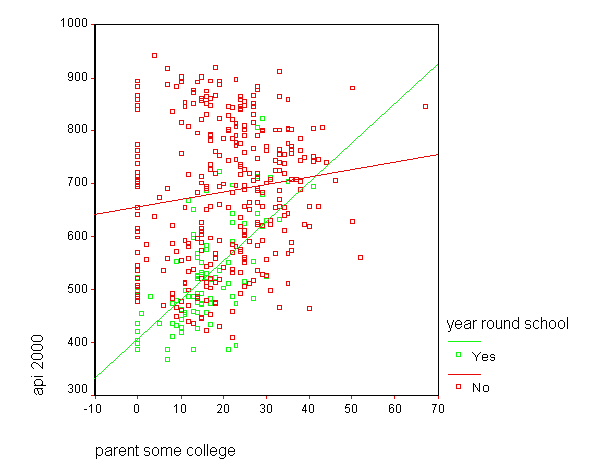
We can replot the same graph including the data points. You will need to double-click on the graph that is produced by the code below to add the regression lines to the graph.
GRAPH
  /SCATTERPLOT(BIVAR)=some_col WITH api00 BY yr_rnd.
Let's quickly run the regressions again where we performed separate regressions for the two groups.
Non-year-round
COMPUTE filt=(yr_rnd=0).
FILTER BY filt.
regress
 /dep = api00
 /method = enter some_col.
| Model | Variables Entered | Variables Removed | Method |
|---|---|---|---|
| 1 | parent some college(a) | . | Enter |
| a All requested variables entered. | |||
| b Dependent Variable: api 2000 | |||
| Model | R | R Square | Adjusted R Square | Std. Error of the Estimate |
|---|---|---|---|---|
| 1 | .126(a) | .016 | .013 | 131.278 |
| a Predictors: (Constant), parent some college | ||||
| Model | Sum of Squares | df | Mean Square | F | Sig. | |
|---|---|---|---|---|---|---|
| 1 | Regression | 84700.858 | 1 | 84700.858 | 4.915 | .027(a) |
| Residual | 5273591.675 | 306 | 17233.960 | |||
| Total | 5358292.532 | 307 | ||||
| a Predictors: (Constant), parent some college | ||||||
| b Dependent Variable: api 2000 | ||||||
| Unstandardized Coefficients | Standardized Coefficients | t | Sig. | |||
|---|---|---|---|---|---|---|
| Model | B | Std. Error | Beta | |||
| 1 | (Constant) | 655.110 | 15.237 | 42.995 | .000 | |
| parent some college | 1.409 | .636 | .126 | 2.217 | .027 | |
| a Dependent Variable: api 2000 | ||||||
Year-round
COMPUTE filt=(yr_rnd=1).
FILTER BY filt.
regress
 /dep = api00
 /method = enter some_col.
| Model | Variables Entered | Variables Removed | Method |
|---|---|---|---|
| 1 | parent some college(a) | . | Enter |
| a All requested variables entered. | |||
| b Dependent Variable: api 2000 | |||
| Model | R | R Square | Adjusted R Square | Std. Error of the Estimate |
|---|---|---|---|---|
| 1 | .648(a) | .420 | .413 | 75.773 |
| a Predictors: (Constant), parent some college | ||||
| Model | Sum of Squares | df | Mean Square | F | Sig. | |
|---|---|---|---|---|---|---|
| 1 | Regression | 373644.064 | 1 | 373644.064 | 65.078 | .000(a) |
| Residual | 516734.838 | 90 | 5741.498 | |||
| Total | 890378.902 | 91 | ||||
| a Predictors: (Constant), parent some college | ||||||
| b Dependent Variable: api 2000 | ||||||
| Unstandardized Coefficients | Standardized Coefficients | t | Sig. | |||
|---|---|---|---|---|---|---|
| Model | B | Std. Error | Beta | |||
| 1 | (Constant) | 407.039 | 16.515 | 24.647 | .000 | |
| parent some college | 7.403 | .918 | .648 | 8.067 | .000 | |
| a Dependent Variable: api 2000 | ||||||
Now, let's show the regression for both types of schools with the interaction term.
filter off.
regress
 /dep = api00
 /method = enter some_col yr_rnd yrXsome
 /save pre.
| Model | Variables Entered | Variables Removed | Method |
|---|---|---|---|
| 1 | YRXSOME, parent some college, year round school(a) | . | Enter |
| a All requested variables entered. | |||
| b Dependent Variable: api 2000 | |||
| Model | R | R Square | Adjusted R Square | Std. Error of the Estimate |
|---|---|---|---|---|
| 1 | .532(a) | .283 | .277 | 120.922 |
| a Predictors: (Constant), YRXSOME, parent some college, year round school | ||||
| b Dependent Variable: api 2000 | ||||
| Model | Sum of Squares | df | Mean Square | F | Sig. | |
|---|---|---|---|---|---|---|
| 1 | Regression | 2283345.485 | 3 | 761115.162 | 52.053 | .000(a) |
| Residual | 5790326.513 | 396 | 14622.037 | |||
| Total | 8073671.997 | 399 | ||||
| a Predictors: (Constant), YRXSOME, parent some college, year round school | ||||||
| b Dependent Variable: api 2000 | ||||||
| Unstandardized Coefficients | Standardized Coefficients | t | Sig. | |||
|---|---|---|---|---|---|---|
| Model | B | Std. Error | Beta | |||
| 1 | (Constant) | 655.110 | 14.035 | 46.677 | .000 | |
| parent some college | 1.409 | .586 | .112 | 2.407 | .017 | |
| year round school | -248.071 | 29.859 | -.735 | -8.308 | .000 | |
| YRXSOME | 5.993 | 1.577 | .330 | 3.800 | .000 | |
| a Dependent Variable: api 2000 | ||||||
| Minimum | Maximum | Mean | Std. Deviation | N | |
|---|---|---|---|---|---|
| Predicted Value | 407.04 | 749.54 | 647.62 | 75.648 | 400 |
| Residual | -275.12 | 279.25 | .00 | 120.466 | 400 |
| Std. Predicted Value | -3.180 | 1.347 | .000 | 1.000 | 400 |
| Std. Residual | -2.275 | 2.309 | .000 | .996 | 400 |
| a Dependent Variable: api 2000 | |||||
Note that the coefficient for some_col in the combined analysis is the same as the coefficient for some_col for the non-year-round schools. This is because non-year-round schools are the reference group. Then, the coefficient for the yrXsome interaction in the combined analysis is the Bsome_col for the year round schools (7.4) minus Bsome_col for the non year round schools (1.41), yielding 5.99. This interaction is the difference in the slopes of some_col for the two types of schools, and this is why this is useful for testing whether the regression lines for the two types of schools are equal. If the two types of schools had the same regression coefficient for some_col, then the coefficient for the yrXsome interaction would be 0. In this case, the difference is significant, indicating that the regression lines are significantly different.
So, if we look at the graph of the two regression lines we can see the difference in the slopes of the regression lines (see graph below). Indeed, we can see that the non-year round schools (the solid line) have a smaller slope (1.4) than the slope for the year round schools (7.4). The difference between these slopes is 5.99, the coefficient for yrXsome.
GRAPH
  /SCATTERPLOT(BIVAR)=some_col WITH pre_1 BY yr_rnd.
3.7.2 Computing interactions with glm
We can also run a model just like the model we showed above using the glm command. We include the terms yr_rnd some_col and the interaction yr_rnr*some_col .
glm
  api00 BY yr_rnd WITH some_col
  /DESIGN = some_col yr_rnd yr_rnd*some_col.
| Value Label | N | ||
|---|---|---|---|
| year round school | 0 | No | 308 |
| 1 | Yes | 92 | |
| Source | Type III Sum of Squares | df | Mean Square | F | Sig. |
|---|---|---|---|---|---|
| Corrected Model | 2283345.485(a) | 3 | 761115.162 | 52.053 | .000 |
| Intercept | 18502483.537 | 1 | 18502483.537 | 1265.383 | .000 |
| SOME_COL | 456473.187 | 1 | 456473.187 | 31.218 | .000 |
| YR_RND | 1009279.986 | 1 | 1009279.986 | 69.025 | .000 |
| YR_RND * SOME_COL | 211143.646 | 1 | 211143.646 | 14.440 | .000 |
| Error | 5790326.513 | 396 | 14622.037 | ||
| Total | 175839633.000 | 400 | |||
| Corrected Total | 8073671.997 | 399 | |||
| a R Squared = .283 (Adjusted R Squared = .277) | |||||
As we illustrated above, we can compute the predicted values using the predict command and graph the separate regression lines. These commands are omitted.
In this section we found that the relationship between some_col and api00 depended on whether the student was from a year-round school or from a non-year-round school. For the students from year- round schools, the relationship between some_col and api00 was significantly stronger than for those from non-year- round schools. In general, this type of analysis allows you to test whether the strength of the relationship between two continuous variables varies based on the categorical variable.
3.8 Continuous and Categorical variables, interaction with 1/2/3 variableThe prior examples showed how to do regressions with a continuous variable and a categorical variable that has 2 levels. These examples will extend this further by using a categorical variable with 3 levels, mealcat.
3.8.1 using regress
We can run a model with some_col mealcat and the interaction of these two variables.
GET FILE='C:spssregelemapi2.sav'.

if mealcat ~= missing(mealcat) mealcat1 = 0.
if mealcat = 1 mealcat1 = 1.
if mealcat ~= missing(mealcat) mealcat2 = 0.
if mealcat = 2 mealcat2 = 1.
if mealcat ~= missing(mealcat) mealcat3 = 0.
if mealcat = 3 mealcat3 = 1.
compute smc1 = mealcat1*some_col.
compute smc2 = mealcat2*some_col.
compute smc3 = mealcat3*some_col.
execute.

regress
 /dep = api00
 /method = enter mealcat2 mealcat3 some_col
 /method = test (smc2 smc3)
 /save pre.
Variables Entered/Removed(b) Model Variables Entered Variables Removed Method 1 parent some college, MEALCAT2, MEALCAT3(a) . Enter 2 SMC3, SMC2 . Test a All requested variables entered. b Dependent Variable: api 2000
Model Summary(c)Model R R Square Adjusted R Square Std. Error of the Estimate 1 .870(a) .757 .756 70.332 2 .877(b) .769 .767 68.733 a Predictors: (Constant), parent some college, MEALCAT2, MEALCAT3 b Predictors: (Constant), parent some college, MEALCAT2, MEALCAT3, SMC3, SMC2 c Dependent Variable: api 2000
ANOVA(d)Model Sum of Squares df Mean Square F Sig. R Square Change 1 Regression 6114838.708 3 2038279.569 412.061 .000(a) Residual 1958833.290 396 4946.549 Total 8073671.997 399 2 Subset Tests SMC2, SMC3 97468.169 2 48734.084 10.316 .000(b) .012 Regression 6212306.876 5 1242461.375 262.995 .000(c) Residual 1861365.121 394 4724.277 Total 8073671.997 399 a Predictors: (Constant), parent some college, MEALCAT2, MEALCAT3 b Tested against the full model. c Predictors in the Full Model: (Constant), parent some college, MEALCAT2, MEALCAT3, SMC3, SMC2. d Dependent Variable: api 2000
Coefficients(a)Unstandardized Coefficients Standardized Coefficients t Sig. Model B Std. Error Beta
1 (Constant) 791.179 9.403 84.143 .000 MEALCAT2 -168.132 8.719 -.556 -19.284 .000 MEALCAT3 -296.436 8.923 -.990 -33.221 .000 parent some college .683 .334 .054 2.043 .042 2 (Constant) 825.894 11.992 68.871 .000 MEALCAT2 -239.030 18.665 -.791 -12.806 .000 MEALCAT3 -344.948 17.057 -1.152 -20.223 .000 parent some college -.947 .487 -.076 -1.944 .053 SMC2 3.141 .729 .286 4.307 .000 SMC3 2.607 .896 .149 2.910 .004 a Dependent Variable: api 2000
Excluded Variables(b)Beta In t Sig. Partial Correlation Collinearity Statistics Model
Tolerance 1 SMC2 .215(a) 3.455 .001 .171 .153 SMC3 .069(a) 1.412 .159 .071 .258 a Predictors in the Model: (Constant), parent some college, MEALCAT2, MEALCAT3 b Dependent Variable: api 2000
Casewise Diagnostics(a)Case Number Std. Residual api 2000 226 -3.593 386 a Dependent Variable: api 2000
Residuals Statistics(a)Minimum Maximum Mean Std. Deviation N Predicted Value 480.95 825.89 647.62 124.779 400 Residual -246.93 201.23 .00 68.301 400 Std. Predicted Value -1.336 1.429 .000 1.000 400 Std. Residual -3.593 2.928 .000 .994 400 a Dependent Variable: api 2000
These results indicate that the overall interaction is indeed significant. This means that the regression lines from the three groups differ significantly. As we have done before, let's the predicted values so we can see how the regression lines differ.
Because we had three groups, we get three regression lines, one for each category of mealcat.
GRAPH
  /LINE(MULTIPLE)MEAN(pre_1) BY some_col BY mealcat.
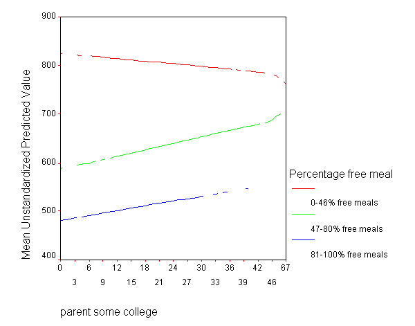
Group 1 was the omitted group, therefore the slope of the line for group 1 is the coefficient for some_col which is -.94. Indeed, this line has a downward slope. If we add the coefficient for some_col to the coefficient for smc2 we get the coefficient for group 2, i.e., 3.14 + -.94 yields 2.2, the slope for group 2. Indeed, group 2 shows an upward slope. Likewise, if we add the coefficient for some_col to the coefficient for smc3 we get the coefficient for group 3, i.e., 2.6 + -.94 yields 1.66, the slope for group 3. So, the slopes for the 3 groups are
group 1: -0.94
group 2:  2.2
group 3:  1.66
The test of the coefficient for smc2 tested whether the coefficient for group 2 differed from group 1, and indeed this was significant. Likewise, the test of the coefficient for smc3 tested whether the coefficient for group 3 differed from group 1, and indeed this was significant. What did the test of the coefficient some_col test? This coefficient represents the coefficient for group 1, so this tested whether the coefficient for group 1 (-0.94) was significantly different from 0. This is probably a non-interesting test.
The comparisons in the above analyses don't seem to be as interesting as comparing group 1 vs. 2 and then comparing group 2 vs. 3. These successive comparisons seem much more interesting. We can do this by making group 2 the omitted group, and then each group would be compared to group 2.
regress
 /dep = api00
 /method = enter mealcat1 mealcat3 some_col smc1 smc3.
| Model | Variables Entered | Variables Removed | Method |
|---|---|---|---|
| 1 | SMC3, parent some college, MEALCAT1, MEALCAT3, SMC1(a) | . | Enter |
| a All requested variables entered. | |||
| b Dependent Variable: api 2000 | |||
| Model | R | R Square | Adjusted R Square | Std. Error of the Estimate |
|---|---|---|---|---|
| 1 | .877(a) | .769 | .767 | 68.733 |
| a Predictors: (Constant), SMC3, parent some college, MEALCAT1, MEALCAT3, SMC1 | ||||
| Model | Sum of Squares | df | Mean Square | F | Sig. | |
|---|---|---|---|---|---|---|
| 1 | Regression | 6212306.876 | 5 | 1242461.375 | 262.995 | .000(a) |
| Residual | 1861365.121 | 394 | 4724.277 | |||
| Total | 8073671.997 | 399 | ||||
| a Predictors: (Constant), SMC3, parent some college, MEALCAT1, MEALCAT3, SMC1 | ||||||
| b Dependent Variable: api 2000 | ||||||
| Unstandardized Coefficients | Standardized Coefficients | t | Sig. | |||
|---|---|---|---|---|---|---|
| Model | B | Std. Error | Beta | |||
| 1 | (Constant) | 586.864 | 14.303 | 41.030 | .000 | |
| MEALCAT1 | 239.030 | 18.665 | .790 | 12.806 | .000 | |
| MEALCAT3 | -105.918 | 18.754 | -.354 | -5.648 | .000 | |
| parent some college | 2.194 | .543 | .175 | 4.043 | .000 | |
| SMC1 | -3.141 | .729 | -.270 | -4.307 | .000 | |
| SMC3 | -.534 | .927 | -.030 | -.576 | .565 | |
| a Dependent Variable: api 2000 | ||||||
Now, the test of smc1 tests whether the coefficient for group 1 differs from group 2, and it does. Then, the test of smc3 tests whether the coefficient for group 3 significantly differs from group 2, and it does not. This makes sense given the graph and given the estimates of the coefficients that we have, that -.94 is significantly different from 2.2 but 2.2 is not significantly different from 1.66.
3.8.2 Using glm
We can perform the same analysis using the glm command, as shown below. The glm command gives us somewhat less flexibility since we cannot choose which group is the omitted group.
GET FILE='C:spssregelemapi2.sav'.
glm
  api00 by mealcat with some_col
  /design = some_col mealcat some_col*mealcat
  /print = parameter TEST(LMATRIX).
| Value Label | N | ||
|---|---|---|---|
| Percentage free meals in 3 categories | 1 | 0-46% free meals | 131 |
| 2 | 47-80% free meals | 132 | |
| 3 | 81-100% free meals | 137 | |
| Source | Type III Sum of Squares | df | Mean Square | F | Sig. |
|---|---|---|---|---|---|
| Corrected Model | 6212306.876(a) | 5 | 1242461.375 | 262.995 | .000 |
| Intercept | 34188885.021 | 1 | 34188885.021 | 7236.850 | .000 |
| SOME_COL | 36366.366 | 1 | 36366.366 | 7.698 | .006 |
| MEALCAT | 2012065.492 | 2 | 1006032.746 | 212.950 | .000 |
| MEALCAT * SOME_COL | 97468.169 | 2 | 48734.084 | 10.316 | .000 |
| Error | 1861365.121 | 394 | 4724.277 | ||
| Total | 175839633.000 | 400 | |||
| Corrected Total | 8073671.997 | 399 | |||
| a R Squared = .769 (Adjusted R Squared = .767) | |||||
| B | Std. Error | t | Sig. | 95% Confidence Interval | ||
|---|---|---|---|---|---|---|
| Parameter | Lower Bound | Upper Bound | ||||
| Intercept | 480.946 | 12.131 | 39.647 | .000 | 457.097 | 504.795 |
| SOME_COL | 1.660 | .752 | 2.208 | .028 | .182 | 3.138 |
| [MEALCAT=1] | 344.948 | 17.057 | 20.223 | .000 | 311.413 | 378.483 |
| [MEALCAT=2] | 105.918 | 18.754 | 5.648 | .000 | 69.046 | 142.789 |
| [MEALCAT=3] | 0(a) | . | . | . | . | . |
| [MEALCAT=1] * SOME_COL | -2.607 | .896 | -2.910 | .004 | -4.369 | -.846 |
| [MEALCAT=2] * SOME_COL | .534 | .927 | .576 | .565 | -1.289 | 2.357 |
| [MEALCAT=3] * SOME_COL | 0(a) | . | . | . | . | . |
| a This parameter is set to zero because it is redundant. | ||||||
<some output omitted to save space>
Because the glm command omits the third category, and the analysis we showed above omitted the second category, the parameter estimates will not be the same. You can compare the results from below with the results above and see that the parameter estimates are not the same. Because group 3 is dropped, that is the reference category and all comparisons are made with group 3.
These analyses showed that the relationship between some_col and api00 varied, depending on the level of mealcat. In comparing group 1 with group 2, the coefficient for some_col was significantly different, but there was no difference in the coefficient for some_col in comparing groups 2 and 3.
3.9 Summary
This chapter covered four techniques for analyzing data with categorical variables, 1) manually constructing indicator variables, 2) using a do-loop, 3) using the regress command, and 4) using the glm command. Each method has its advantages and disadvantages, as described below.
Manually constructing indicator variables can be very tedious and even error prone. For very simple models, it is not very difficult to create your own indicator variables, but if you have categorical variables with many levels and/or interactions of categorical variables, it can be laborious to manually create indicator variables. However, the advantage is that you can have quite a bit of control over how the variables are created and the terms that are entered into the model.
A do-loop will allow you to create many indicator variables very quickly. However, there are some restrictions regarding the naming of the variables and all of the variables must have the same two values (i.e., zero and one or one and two).
The regress command is useful when you want to test one or a group of variables together.
The glm command is useful for those times when you want to use a particular coding scheme to perform certain types of tests, such as comparing each level of a variable to the previous level. The glm command in SPSS will create the appropriate codes for the variables and display the coding scheme in the output.
3.10 For more information
See the following web pages for more information and resources on regression with categorical predictors in SPSS.
- SPSS FAQ- How do I interpret the parameter estimates for dummy variables
- SPSS FAQ- How can I compare regression coefficients between 2 groups
- SPSS FAQ- How can I compare regression coefficients across 3 or more groups
- SPSS Textbook Examples- Applied Regression Analysis, Chapter 7
- SPSS Library- How do I handle interactions of continuous and categorical variables in regression
- SPSS Library- Understanding and Interpreting Parameter estimates in Regression and Anova