This is a draft version of this chapter. Comments and suggestions to improve this draft are welcome.
Chapter Outline
6.1. Analysis with 2 categorical variables
6.2. Simple effects
6.2.1 Analyzing Simple Effects Using MANOVA and GLM
6.2.2 Analyzing Simple Effects Using REGRESSION
6.3. Simple Comparisons
6.3.1 Analyzing Simple Comparisons Using MANOVA and GLM
6.3.2 Analyzing Simple Comparisons Using REGRESSION
6.4. Partial Interaction
6.4.1 Analyzing partial interactions Using MANOVA and GLM
6.4.2 Analyzing partial interactions Using REGRESSION
6.5. Interaction contrasts
6.5.1 Analyzing interaction contrasts using MANOVA and GLM
6.5.2 Analyzing interaction contrasts using REGRESSION
6.6 Computing Adjusted Means
6.6.1 Computing Adjusted Means via MANOVA and GLM
6.6.2 Computing
Adjusted Means via REGRESSION
6.7 More Details on Meaning of the Coefficients
6.8 Simple Effects via Dummy Coding vs. Effect Coding
6.8.1 Example 1. Simple effects of yr_rnd at levels of mealcat
6.8.2 Example 2. Simple effects of mealcat at levels of yr_rnd
For this chapter we will use the elemapi2 data file that we have been using in prior chapters. We will focus on the variables mealcat, and collcat as they relate to the outcome variable api00 (performance on the api in the year 2000. The variable mealcat is the variable meals broken up into 3 categories, and the variable collcat is the variable some_col broken into 3 categories. We could think of mealcat as being the number of students receiving free meals and broken up into low, middle and high. The variable collcat can be thought of as the number of parents with some college education, and we could think of it as being broken up into low, medium and high. For our analysis, we think that both mealcat and collcat may be related to api00, but it is also possible that the impact of mealcat might depend on the level of collcat. In other words, we think that there might be an interaction of these two categorical variables. In this chapter we will look at how these two categorical variables are related to api performance in the school, and we will look at the interaction of these two categorical variables as well. We will see that there is an interaction of these categorical variables, and will focus on different ways of further exploring the interaction.
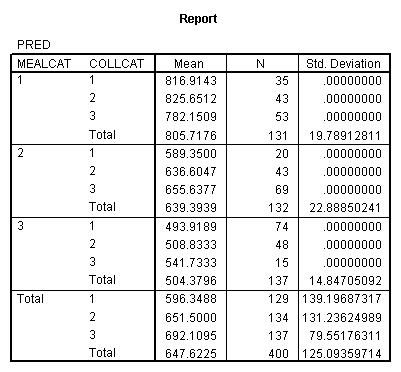
We will first input the elemapi2 data file and have a quick look at the three variables we are interested in.
get file = "c:spssregelemapi2.sav".means tables= api00 by mealcat by collcat /cells=mean.
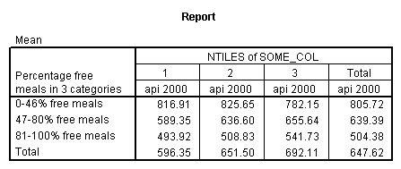
We drop the label for mealcat because this can get in the way at some of the points we will be demonstrating.
value labels mealcat.
6.1. Analysis with 2 categorical variables
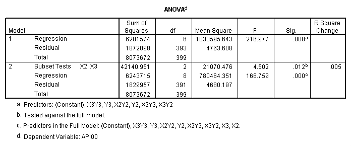
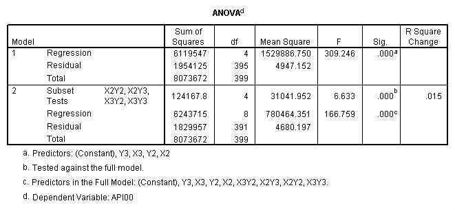
One traditional way to analyze this would be to perform a 3 by 3 factorial analysis of variance using the glm command, as shown below. The results show a main effect of collcat (F=4.5, p-0.0117), a main effect of mealcat (F=509.04, p=0.0000) and an interaction of collcat by mealcat, (F=6.63, p=0.0000).
glm
api00 by collcat mealcat
/plot = profile( mealcat*collcat )
/emmeans = tables(collcat*mealcat).
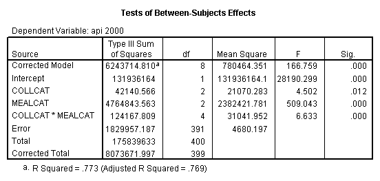
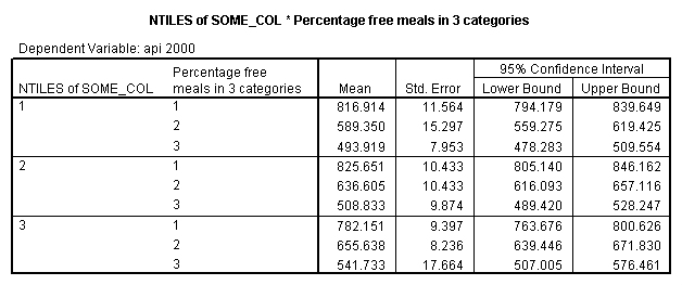
The option emmeans (which stands for Estimated Marginal Means) gives the adjusted means broken down by collcat and mealcat shown below.
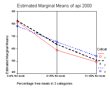
We can show a graph of the adjusted means as shown below. This is done with the option plot in glm procedure.
We can do these same analyses using the regress command. Below we first create simple regression coding for both variables collcat and mealcat. Then we use the regression procedure based on those variables.
recode collcat (1=-.66667)  (2=.33333)  (3=.33333)  into  x2.
recode collcat (1=.33333)  (2=-.66667)  (3=.33333)  into  x3.

recode mealcat (1=-.66667)  (2=.33333)  (3=.33333) into y2.
recode mealcat (1= .33333)  (2=-.66667) (3=.33333) into y3.

compute x2y2 = x2*y2.
compute x2y3 = x2*y3.
compute x3y2 = x3*y2.
compute x3y3 = x3*y3.
execute .

regression
/dependent api00
/method=enter x2 x3 y2 y3 x2y2 x2y3 x3y2 x3y3.
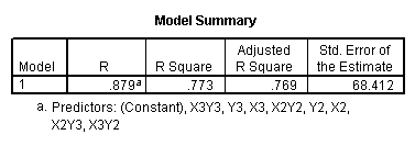

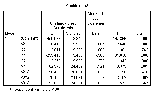
We use the test command to test the two terms associated with collcat to get the main effect of collcat.
regression
/dependent api00
/method=enter y2 y3 x2y2 x2y3 x3y2 x3y3
/method = test(x2 x3).
Likewise we use the test command to get the test on main effect of mealcat.
regression
/dependent api00
/method=enter x2 x3 x2y2 x2y3 x3y2 x3y3
/method = test(y2 y3).
Finally, we use the test command to test the interaction of of collcat by mealcat.
regression
/dependent api00
/method=enter x2 x3 y2 y3
/method = test(x2y2 x2y3 x3y2 x3y3).
First, note that the results of the test commands correspond to those from the glm command above. This is because collcat and mealcat were coded using simple effect coding, a coding scheme where the contrasts sum to 0. If this had been coded using dummy coding, then the results of the test commands for mealcat and collcat from the regress command would not have corresponded to the glm results. In addition to simple coding, we could have used deviation or helmert coding schemes and the results of the test commands would have matched with the anova result from glm command, although the meaning of the individual tests would have been different. This point will be explored in more detail later in this chapter.
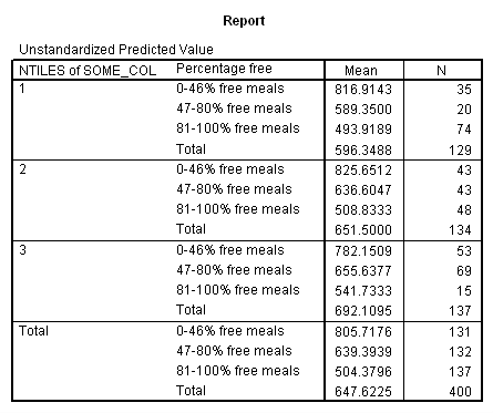
We can obtain the adjusted means by using predict command to get the predicted values, calling them pred and then looking at the mean of pred broken down by collcat and mealcat.
regression
  /dependent api00
  /method=enter x2 x3 x2y2 x2y3  x3y2 x3y3  y2 y3
  /save pred(pred).

means
  pred  by mealcat by collcat.
The graph of the cell means from glm procedure illustrates the interaction between collcat and mealcat. The graph shows the 3 levels of collcat as 3 different lines, and the 3 levels of mealcat as the 3 values on the x axis of the graph. We can see that the effect of collcat differs based on the level of mealcat. For example, when mealcat is low, schools where collcat is 3 have the lowest api00 scores, as compared to schools that are medium or high on mealcat, where schools with collcat of 3 have the highest api00 scores.
Let’s investigate this interaction further by looking at the simple effects of collcat at each level of mealcat.
6.2. Simple effects
We found that the main effect of collcat was significant, but because we have an interaction the effect of collcat depends on the level of mealcat. We might want to ask whether the effect of collcat is significant at each level of mealcat.
6.2.1 Analyzing Simple Effects Using MANOVA and GLM
In SPSS, we can use either MANOVA procedure or GLM procedure in order to look at the simple effects of a variable. For example, in order to look at the simple effect of collcat at the different levels of mealcat, we can use the following MANOVA statement.
manova api00 by collcat(1,3) mealcat(1,3)
  /error =  w
  /design = mealcat
                collcat within mealcat(1)
                collcat within mealcat(2)
                collcat within mealcat(3).
* * * * * * A n a l y s i s o f V a r i a n c e * * * * * * 400 cases accepted. 0 cases rejected because of out-of-range factor values. 0 cases rejected because of missing data. 9 non-empty cells. 1 design will be processed. * * * * * * A n a l y s i s o f V a r i a n c e -- design 1 * * * * Tests of Significance for API00 using UNIQUE sums of squares Source of Variation SS DF MS F Sig of F WITHIN CELLS 1829957.19 391 4680.20 MEALCAT 4764843.56 2 2382421.8 509.04 .000 COLLCAT WITHIN MEALC 50909.25 2 25454.62 5.44 .005 AT(1) COLLCAT WITHIN MEALC 68628.74 2 34314.37 7.33 .001 AT(2) COLLCAT WITHIN MEALC 29979.15 2 14989.57 3.20 .042 AT(3) (Model) 6243714.81 8 780464.35 166.76 .000 (Total) 8073672.00 399 20234.77 R-Squared = .773 Adjusted R-Squared = .769
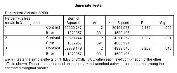
we can also use glm procedure with the emmeans statement. We can obtain the simple effect of collcat at each level of mealcat using the compare option. This shows that the effect of collcat at each level of mealcat.
glm api00 by collcat mealcat
/emmeans tables(collcat*mealcat) compare(collcat).
This shows that collcat is significant at each level of mealcat , if we use an alpha level of 0.05. We should note that since we are doing a number of additional tests, you might want to consider using post hoc corrections, such as a bonferoni correction to avoid Type I errors.
In summary, all 3 of the simple effects of collcat at each level of mealcat were significant, however the effect of collcat when mealcat was 3 might not be significant if we used a post hoc criteria for evaluating its significance.
6.2.2 Analyzing Simple Effects Using REGRESSION
We have demonstrated how to test the simple effect of collcat at each level of mealcat using GLM procedure in the previous section. That is through the approach of ANOVA. We can also obtain the same analysis through regression approach. After all, Anova is regression. In regression approach, we will create the coding for variable collcat, mealcat and their interaction. The coding scheme is specific for the effect we want to see. For example, in this section, we will do an analysis parallel to the previous section. That is to say that we want to see the simple effect of collcat at each level of mealcat. We will use simple coding for mealcat, though in our case the type of coding for mealcat does not really matter. The scheme for simple coding is shown chapter 5. The reference group for mealcat is group 1.
recode mealcat (1=.33333)  (2=.33333)  (3=-.66667)  into mcat1.
recode mealcat (1= .33333) (2=-.66667)  (3=.33333)  into mcat2.
We use helmert coding for collcat. We should note that these terms are not used in the analysis, but are used for creating the simple effects of collcat at each level of mealcat.
recode collcat (1=.66667)  (2=-.33333)  (3=-.33333)  into  ccat1.
recode collcat (1=0)  (2=.5)  (3=-.5) into  ccat2.

compute c1m1 = 0.
compute c2m1 = 0.
compute c1m2 = 0.
compute c2m2 = 0.
compute c1m3 = 0.
compute c2m3 = 0.

 if ( mealcat = 1)  c1m1 = ccat1.
 if ( mealcat = 1)  c2m1 = ccat2.

 if ( mealcat = 2)  c1m2 = ccat1.
 if ( mealcat = 2)  c2m2 = ccat2.

 if ( mealcat = 3)  c1m3 = ccat1.
 if ( mealcat = 3)  c2m3 = ccat2.
Now, that we have seen the helmert coding for collcat, we can see how this is used to create the simple effects of collcat at each level of mealcat. First, we look at the two comparisons of collcat at mealcat of 1. Note that the coding is the same as we saw above, but only when mealcat is 1, otherwise these variables are coded 0. Likewise, we look at the terms that form the effects of collcat when mealcat is 2, and we see that the variables are coded the same way when mealcat is 2, and otherwise 0. The same is true for the case when mealcat is 3. The following matrix is the coding we just used for all the interaction terms.
| collcat | mealcat | c1m1 | c2m1 | c1m2 | c2m2 | c1m3 | c2m3 |
| 1 | 1 | 2/3 | 0 | 0 | 0 | 0 | 0 |
| 2 | 1 | -1/3 | 1/2 | 0 | 0 | 0 | 0 |
| 3 | 1 | -1/3 | -1/2 | 0 | 0 | 0 | 0 |
| 1 | 2 | 0 | 0 | 2/3 | 0 | 0 | 0 |
| 2 | 2 | 0 | 0 | -1/3 | 1/2 | 0 | 0 |
| 3 | 2 | 0 | 0 | -1/3 | -1/2 | 0 | 0 |
| 1 | 3 | 0 | 0 | 0 | 0 | 2/3 | 0 |
| 2 | 3 | 0 | 0 | 0 | 0 | -1/3 | 1/2 |
| 3 | 3 | 0 | 0 | 0 | 0 | -1/3 | -1/2 |
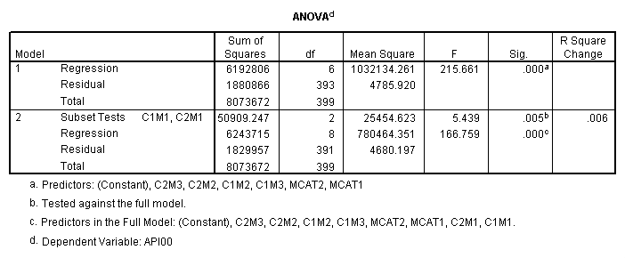
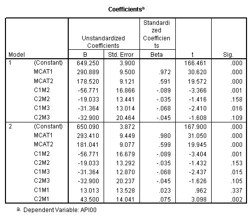
Now we are ready for our regression analysis. The test statement used below is for testing the simple effect of collcat at mealcat = 1.
regression
/dependent api00
/method=enter mcat1 mcat2 c1m2 c2m2 c1m3 c2m3
/method = test(c1m1 c2m1).
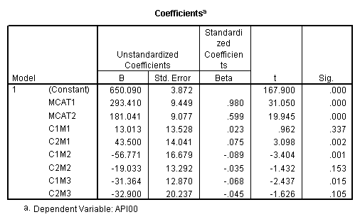
We now see the simple effect of collcat when mealcat = 1 from the ANOVA output and we also see the regression estimates from the regression table. This illustrates how we have coded variables to allow the simple effects analysis. We can get the same analysis for the case when mealcat is 2 or 3 using different test statements. If you wished, you could manually create variables according to this strategy to perform a simple effects analysis.
6.3 Simple Comparisons
In the analyses above we looked at the simple effect of collcat at each level of mealcat. For example, we looked at the overall effect of collcat when mealcat was 1. This is the simple effect of collcat at mealcat=1. Because collcat has more than 2 levels, we may wish to make further comparisons among the 3 levels of collcat within mealcat=1. Simple comparisons allow us to make such comparisons.
6.3.1 Analyzing Simple Comparisons Using MANOVA and GLM
We can also look at the simple comparisons either using MANOVA or GLM as we did in Section 6.2. First we look at the comparison of collcat 1 vs. 2 and 3 when mealcat is 1 and then at the comparison of collcat 2 vs. 3. Let’s look at the MANOVA code first and its output first.
manova api00 by collcat(1,3) mealcat(1,3)
  /error =  w
  /contrast (collcat)=helmert
  /design = mealcat
                collcat within mealcat(1)
                collcat within mealcat(2)
                collcat within mealcat(3).

* * * * * * A n a l y s i s   o f   V a r i a n c e * * * * * *

       400 cases accepted.
         0 cases rejected because of out-of-range factor values.
         0 cases rejected because of missing data.
         9 non-empty cells.

         1 design will be processed.

* * * * * * A n a l y s i s   o f   V a r i a n c e -- design   1 * * * * * *

 Tests of Significance for API00 using UNIQUE sums of squares
 Source of Variation          SS      DF        MS         F  Sig of F

 WITHIN CELLS         1829957.19     391   4680.20
 MEALCAT              4764843.56       2 2382421.8    509.04      .000
 COLLCAT WITHIN MEALC   50909.25       2  25454.62      5.44      .005
 AT(1)
 COLLCAT WITHIN MEALC   68628.74       2  34314.37      7.33      .001
 AT(2)
 COLLCAT WITHIN MEALC   29979.15       2  14989.57      3.20      .042
 AT(3)

 (Model)              6243714.81       8 780464.35    166.76      .000
 (Total)              8073672.00     399  20234.77

 R-Squared =           .773
 Adjusted R-Squared =  .769

 - - - - - - - - - - - - - - - - - - - - - - - - - - - - - - - - - - - - -
 Estimates for API00
 --- Individual univariate .9500 confidence intervals

 MEALCAT

  Parameter     Coeff.  Std. Err.    t-Value     Sig. t Lower -95%  CL- Upper
        2   158.150541    5.21975   30.29846     .00000  147.88824  168.41284
        3   -22.890813    5.49562   -4.16528     .00004  -33.69548  -12.08614

 COLLCAT WITHIN MEALCAT(1)

  Parameter     Coeff.  Std. Err.    t-Value     Sig. t Lower -95%  CL- Upper
        4   13.0132326   13.52800     .96195     .33667  -13.58349   39.60995
        5   43.5002194   14.04092    3.09810     .00209   15.89507   71.10536

 COLLCAT WITHIN MEALCAT(2)

  Parameter     Coeff.  Std. Err.    t-Value     Sig. t Lower -95%  CL- Upper
        6   -56.771166   16.67866   -3.40382     .00073  -89.56223  -23.98010
        7   -19.033030   13.29175   -1.43194     .15296  -45.16528    7.09922

 COLLCAT WITHIN MEALCAT(3)

  Parameter     Coeff.  Std. Err.    t-Value     Sig. t Lower -95%  CL- Upper
        8   -31.364414   12.86955   -2.43710     .01525  -56.66658   -6.06225
        9   -32.900000   20.23653   -1.62577     .10480  -72.68603    6.88603
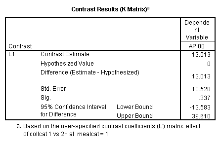
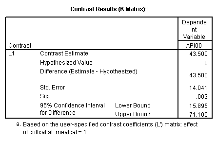
Since we only look at the comparison when mealcat is 1, we only look at the section of the output for COLLCAT WITHIN MEALCAT(1). Parameter 4 is the comparison of collcat 1 vs. 2 and 3 and parameter 5 is the comparison of collcat 2 vs. 3. We see that the collcat 1 is not significantly different from 2 and 3 at mealcat =1 since the t-value is .96 and the p-value is .337, but collcat 2 is significantly different from 3 at mealcat =1 with t-value = 3.10 and p-value = .0021.
Now we will use GLM to get the same results. With GLM, we have to use the lmatrix statement and manually put the helmert coding in. Since we are only interested in the comparison of collcat 1 vs. 2 and 3 at mealcat =1, we leave the last two columns for the interaction collcat*mealcat to be zero because they correspond to the level of 2 and 3 of mealcat.
glm api00 by collcat mealcat
  /lmatrix = 'effect of collcat 1 vs 2+ at mealcat = 1'
                                 collcat 1  -1/2  -1/2
                         collcat*mealcat 1    0     0
                                       -1/2   0     0
                                       -1/2   0     0.
glm api00 by collcat mealcat
  /lmatrix= 'collcat 2 vs. 3 at mealcat = 1'  collcat  0   1  -1
                                      collcat*mealcat  0   0   0
                                                       1   0   0
                                                      -1   0   0.
6.3.2 Analyzing Simple Comparisons Using REGRESSION
In the analyses above we used helmert coding for collcat. We chose this coding so we could compare group 1 with groups 2 and 3 and then compare groups 2 and 3. For example, if we wanted to compare collcat 1 vs. 2 and 3, we would want to look at the effect c1m1, and if we wanted to compare collcat groups 2 and 3 when mealcat is 1, then we would look at the effect c2m1.
We can use the REGRESSION procedure as above to see the effects for these terms.
regression
/dependent api00
/method=enter mcat1 mcat2 c1m1 c2m1 c1m2 c2m2 c1m3 c2m3.
We see that the collcat 1 is not significantly different from 2&3 at mealcat 1 (t=.96, p=.337), but collcat 2 is significantly different from 3 at mealcat 1 (t=3.10, p=0.002).
6.4. Partial Interaction
A partial interaction allows you to apply contrasts to one of the effects in an interaction term. For example, we can draw the interaction of collcat by mealcat like this below.
| Collcat low | Collcat Med | Collcat High | |
| Mealcat Low | |||
| Mealcat Med | |||
| Mealcat High |
Say that we wanted to compare, in the context of this interaction, group 1 for collcat vs. groups 2 and 3. The table of this partial interaction would look like this. The contrast coefficients of -2 1 1 applied to collcat indicate the comparison of group 1 for collcat vs. groups 2 and 3.
| -2 | 1 | 1 | |
| Collcat low | Collcat Med | Collcat High | |
| Mealcat Low | |||
| Mealcat Med | |||
| Mealcat High |
Likewise, we also might want to compare groups 2 and 3 of collcat by mealcat, and the table of this interaction would look like this.
| 0 | -1 | 1 | |
| Collcat low | Collcat Med | Collcat High | |
| Mealcat Low | |||
| Mealcat Med | |||
| Mealcat High |
These are called partial interactions because contrast coefficients are applied to one of the terms involved in the interaction.
6.4.1 Analyzing partial interactions Using MANOVA and GLM
The MANOVA handles partial interaction quite easily. We are interested in the partial interaction of collcat comparing 1 vs. 2 and 3 by mealcat. So we have the helmert coding for collcat. collcat(1) is to compare collcat 1 vs. 2 and 3 and collcat(2) is to compare collcat 2 vs. 3.
manova api00 by collcat(1,3) mealcat(1,3)
/error = w
/contrast(collcat) = helmert
/design =  collcat
           mealcat
           collcat(1) by mealcat
           collcat(2) by mealcat.


* * * * * * A n a l y s i s   o f   V a r i a n c e * * * * * *


       400 cases accepted.
         0 cases rejected because of out-of-range factor values.
         0 cases rejected because of missing data.
         9 non-empty cells.

         1 design will be processed.

* * * * * * A n a l y s i s   o f   V a r i a n c e -- design   1 * * * * * *

 Tests of Significance for API00 using UNIQUE sums of squares
 Source of Variation          SS      DF        MS         F  Sig of F

 WITHIN CELLS         1829957.19     391   4680.20
 COLLCAT                42140.57       2  21070.28      4.50      .012
 MEALCAT              4764843.56       2 2382421.8    509.04      .000
 COLLCAT(1) BY MEALCA   54141.41       2  27070.70      5.78      .003
 COLLCAT(2) BY MEALCA   66511.60       2  33255.80      7.11      .001

 (Model)              6243714.81       8 780464.35    166.76      .000
 (Total)              8073672.00     399  20234.77

 R-Squared =           .773
 Adjusted R-Squared =  .769

 - - - - - - - - - - - - - - - - - - - - - - - - - - - - - - - - - - - - -
 Estimates for API00
 --- Individual univariate .9500 confidence intervals

 COLLCAT

  Parameter     Coeff.  Std. Err.    t-Value     Sig. t Lower -95%  CL- Upper
        2   -25.040783    8.34539   -3.00055     .00287  -41.44823   -8.63333
        3   -2.8109369    9.32938    -.30130     .76335  -21.15296   15.53108

 MEALCAT

  Parameter     Coeff.  Std. Err.    t-Value     Sig. t Lower -95%  CL- Upper
        4   158.150541    5.21975   30.29846     .00000  147.88824  168.41284
        5   -22.890813    5.49562   -4.16528     .00004  -33.69548  -12.08614

 COLLCAT(1) BY MEALCAT

  Parameter     Coeff.  Std. Err.    t-Value     Sig. t Lower -95%  CL- Upper
        6   38.0540153   11.43013    3.32927     .00095   15.58182   60.52621
        7   -31.730384   12.74250   -2.49012     .01318  -56.78278   -6.67799

 COLLCAT(2) BY MEALCAT

  Parameter     Coeff.  Std. Err.    t-Value     Sig. t Lower -95%  CL- Upper
        8   46.3111563   12.35933    3.74706     .00021   22.01210   70.61022
        9   -16.222093   12.08005   -1.34288     .18009  -39.97206    7.52788
Looking at the output of Analysis of Variance, we see that the effect of collcat(1) is significant by mealcat. That means we have this partial interaction is significant. Similarly, we can look at the effect of collcat(2) from the output of Analysis of Variance and it is also significant.
With procedure GLM, we can test the partial interactions using the lmatrix statement. For example, we want to test the partial interaction of collcat comparing group 1 vs. 2 and 3 by mealcat, we can do the following lmatrix statement. Because mealcat has 2 degree of freedom, the test of partial interaction also has 2 degree of freedom. The 2 degree of freedom of factor mealcat can be broken down into 2 comparisons. These two interaction contrasts are separated by a semi-colon, which tells SPSS to join these contrasts together into a single test with 2 degrees of freedom.
glm api00 BY collcat mealcat
  /lmatrix = 'collcat 1 vs.2+ by mealcat' collcat*mealcat   -1  0     1
                             				   1/2  0  -1/2
                               				   1/2  0  -1/2;
                          		  collcat*mealcat   0  -1     1
                              				    0  1/2   -1/2
				                            0  1/2   -1/2.
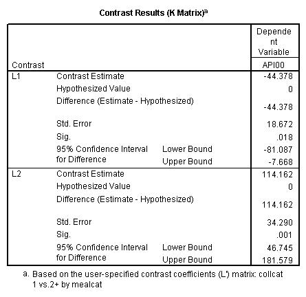

Similarly, we can test the two terms of interaction that involve the comparison of group 2 vs. 3 on collcat. We omit the syntax and the output here.
6.4.2 Analyzing partial interactions Using REGRESSION
With regression analysis, we can also compare groups 1 vs. 2 and 3 on collcat, or compare groups 2 and 3 on collcat. This implies Helmert coding on collcat, as we did before.
recode collcat (1=.66667)  (2=-.33333)  (3=-.33333)  into  ccat1 .
recode collcat (1=0)  (2=.5)  (3=-.5) into  ccat2 .
The coding for mealcat is chosen as dummy coding, but could have been any form of effect coding.
recode mealcat (1=1)  (2=0)  (3=0)  into  md1.
recode mealcat (1=0)  (2=1)  (3=0)  into  md2.
The interaction terms are just the product of their respective main effects.
compute c1m1 = ccat1*md1.
compute c2m1 = ccat2*md1.
compute c1m2 = ccat1*md2.
compute c2m2 = ccat2*md2.
execute.
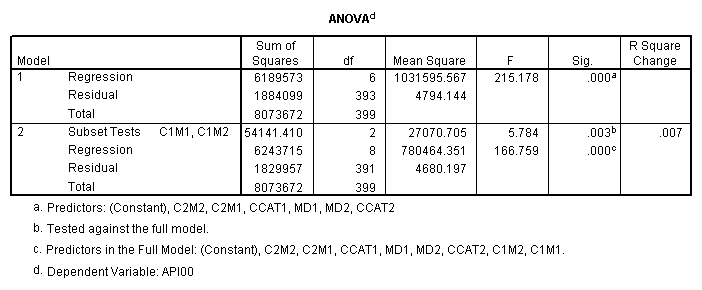
Under such coding scheme, the comparison of collcat 1 vs. 2 and 3 at mealcat 3 is simply ccat1, the comparison of collcat 1 vs. 2 and 3 at mealcat 1 is ccat1 + c1m1 and at mealcat 2 is ccat1 + c1m2. Therefore, to compare collcat group1 vs. group 2 and 3 across all levels of mealcat is the same as testing c1m1 = 0 and c1m2 = 0 simultaneously. Here is the regression with the test.
regression
/dependent api00
/method=enter ccat1 ccat2 md1 md2 c2m1 c2m2
/method = test(c1m1 c1m2).
6.5. Interaction contrasts
Above we saw that a partial interaction allows you to apply contrast coefficients to one of the terms in a 2 way interaction. An interaction contrast allows you to apply contrast coefficients to both of the terms in a two way interaction.
For example, with respect to collcat, let’s say that we wish to compare groups 2 and 3, and with respect to mealcat we wish to compare groups 1 and 2. The table of this looks like this below.
| -1 | 1 | 0 | ||
| Collcat low | Collcat Med | Collcat High | ||
| 0 | Mealcat Low | |||
| -1 | Mealcat Med | |||
| 1 | Mealcat High | |||
We also would like to form a second interaction contrast that also compares groups 2 and 3 with respect to collcat, and compares groups 2 and 3 on mealcat. A table of this comparison is shown below.
| 0 | -1 | 1 | ||
| Collcat low | Collcat Med | Collcat High | ||
| 0 | Mealcat Low | |||
| -1 | Mealcat Med | |||
| 1 | Mealcat High | |||
If we look at the graph of the predicted values (repeated below) we constructed before, it compares the dashed and dotted lines (collcat 2 vs. 3) by mealcat 1 vs. 2, and then again by mealcat 2 vs. 3.

6.5.1 Analyzing interaction contrasts using MANOVA and GLM
Because we would like to compare groups 1 vs. 2, and then groups 2 vs. 3 on mealcat, this implies forward difference coding for mealcat (which will compare 1 vs. 2, then 2 vs. 3). In SPSS, the forward difference coding is called repeated. For collcat we wish to compare groups 2 and 3, so we can use Helmert coding for that comparison as we did above (since this will compare 1 vs. 2 and 3, then 2 vs. 3).
manova api00 by collcat(1, 3)  mealcat(1,3)
/analysis api00
/error = w
/contrast  (collcat) = helmert
/contrast (mealcat) = repeated
/design = collcat, mealcat, collcat by mealcat.
* * * * * * A n a l y s i s o f V a r i a n c e -- design 1 * * * * * * Tests of Significance for API00 using UNIQUE sums of squares Source of Variation SS DF MS F Sig of F WITHIN CELLS 1829957.19 391 4680.20 COLLCAT 42140.57 2 21070.28 4.50 .012 MEALCAT 4764843.56 2 2382421.8 509.04 .000 COLLCAT BY MEALCAT 124167.81 4 31041.95 6.63 .000 (Model) 6243714.81 8 780464.35 166.76 .000 (Total) 8073672.00 399 20234.77 R-Squared = .773 Adjusted R-Squared = .769 - - - - - - - - - - - - - - - - - - - - - - - - - - - - - - - - - - - - - Estimates for API00 --- Individual univariate .9500 confidence intervals COLLCAT Parameter Coeff. Std. Err. t-Value Sig. t Lower -95% CL- Upper 2 -25.040783 8.34539 -3.00055 .00287 -41.44823 -8.63333 3 -2.8109369 9.32938 -.30130 .76335 -21.15296 15.53108 MEALCAT Parameter Coeff. Std. Err. t-Value Sig. t Lower -95% CL- Upper 4 181.041353 9.07713 19.94479 .00000 163.19527 198.88743 5 112.368916 9.90759 11.34170 .00000 92.89009 131.84774 COLLCAT BY MEALCAT Parameter Coeff. Std. Err. t-Value Sig. t Lower -95% CL- Upper 6 69.7843988 21.47520 3.24953 .00126 27.56308 112.00571 7 -25.406752 21.06663 -1.20602 .22854 -66.82479 16.01128 8 62.5332494 19.33438 3.23430 .00132 24.52090 100.54560 9 13.8669700 24.21132 .57275 .56714 -33.73369 61.46763
Since we have chosen Helmert coding for collcat and forward difference coding for mealcat, the interaction terms are coded in the following way. Parameter 6 is for
collcat (1 vs. 2+) & mealcat (1 vs. 2), parameter 7 is for collcat (1 vs. 2+) & mealcat (2 vs. 3), parameter 8 is for collcat (2 vs. 3) & mealcat (1 vs. 2) and parameter 9 is for collcat (2 vs. 3) & mealcat (2 vs. 3).
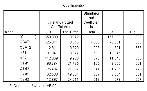
Remember that our first interest is to compare collcat groups 2 and 3, and with respect to mealcat we wish to compare groups 1 and 2.This is tested by parameter 8 , and this term is significant. As we expect, the red and green lines are not parallel when we compare mealcat 1 and 2.
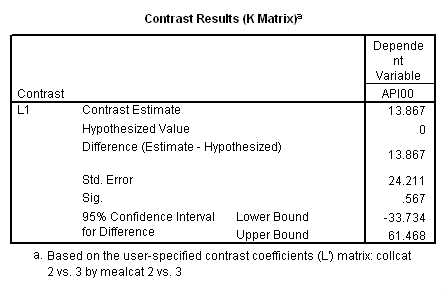
Our second interest is to compares groups 2 and 3 with respect to collcat, and compares groups 2 and 3 on mealcat. This is tested by parameter 9, and this term is not significant. Looking at the graph, we can see that the red and green lines are mostly parallel between mealcat 2 and 3.
We can also get the same analysis using GLM procedure. For example, in our first interaction effect analysis, we compare collcat group 2 vs. 3, and with respect to mealcat we compare groups 1 and 2, this leads to a column matrix for the effect of collcat as (0 1 -1)’ and a row matrix for the effect of mealcat (1 -1 0). This yields the lmatrix shown below.
glm api00 by collcat mealcat
/lmatrix = 'collcat 2 vs. 3 by mealcat 1 vs. 2'
           collcat*mealcat 0 0 0 1 -1 0 -1 1 0.
In the same way, we will get our second analysis from the following.
glm api00 by collcat mealcat
/lmatrix = 'collcat 2 vs. 3 by mealcat 2 vs. 3'
           collcat*mealcat 0 0 0 0 1 -1 0 -1 1.
6.5.2
Analyzing interaction contrasts using REGRESSION
In regression analysis, we have seen that difference coding schemes of the variables give us difference contrasts and comparisons. Because we would like to compare groups 1 vs. 2, and then groups 2 vs. 3 on mealcat, we will use forward difference coding for mealcat (which will compare 1 vs. 2, then 2 vs. 3).
recode mealcat (1=.66667)  (2=-.33333)  (3=-.33333) into mf1.
recode mealcat (1=.33333)  (2=.33333)  (3=-.66667)  into mf2.

compute c1m1 = ccat1*mf1.
compute c2m1 = ccat2*mf1.
compute c1m2 = ccat1*mf2.
compute c2m2 = ccat2*mf2.
execute.
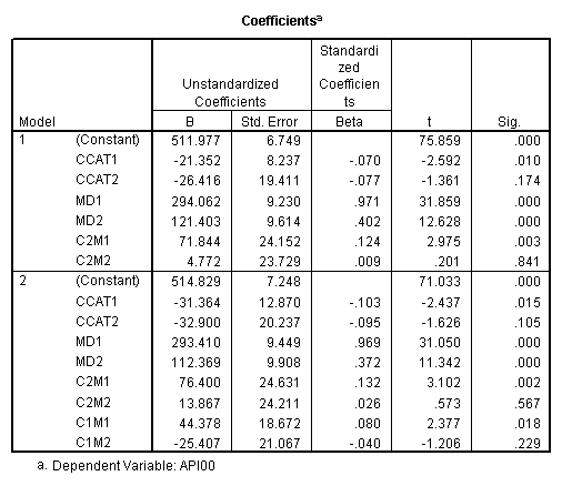
The regression analysis is then done and we can look at the coefficients for c2m1 and c2m2 to see the two comparisons that we have seen from the previous section.
regression
/dependent api00
/method=enter ccat1 ccat2 mf1 mf2 c1m1 c1m2 c2m1 c2m2.
6.6 Computing Adjusted Means
6.6.1 Computing Adjusted Means via MANOVA and GLM
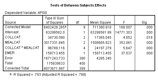
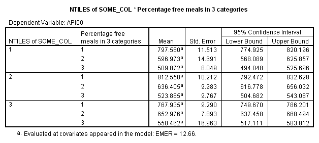
First, we show how you can compute adjusted means using the MANOVA command. Our model will be almost the same as before, in addition we include an additional covariate emer. MANOVA’s option pmeans handles adjusted means for us. These adjusted means compute the mean that would be expected if every school in the sample were at the mean for the variable emer. The syntax to get the adjusted means using manova is as follows. The last table from the output is the adjusted means adjusted by the mean of emer, called combined adjusted means in SPSS.
manova api00 by collcat(1,3) mealcat(1,3) with emer
/analysis api00 with emer
/pmeans tables(collcat*mealcat).


* * * * * * A n a l y s i s   o f   V a r i a n c e -- design   1 * * * * * *

 Order of Variables for Analysis

   Variates     Covariates

    API00         EMER

    1 Dependent Variable
    1 Covariate

* * * * * * A n a l y s i s   o f   V a r i a n c e -- design   1 * * * * * *

 Tests of Significance for API00 using UNIQUE sums of squares
 Source of Variation          SS      DF        MS         F  Sig of F

 WITHIN CELLS         1671243.73     390   4285.24
 REGRESSION            158713.45       1 158713.45     37.04      .000
 COLLCAT                34730.09       2  17365.04      4.05      .018
 MEALCAT              3017331.85       2 1508665.9    352.06      .000
 COLLCAT BY MEALCAT     96789.12       4  24197.28      5.65      .000

 (Model)              6402428.26       9 711380.92    166.01      .000
 (Total)              8073672.00     399  20234.77

 R-Squared =           .793
 Adjusted R-Squared =  .788

 - - - - - - - - - - - - - - - - - - - - - - - - - - - - - - - - - - - - -
 Regression analysis for WITHIN CELLS error term
 --- Individual Univariate .9500 confidence intervals
 Dependent variable .. API00             api 2000

 COVARIATE            B        Beta   Std. Err.     t-Value   Sig. of t

 EMER          -2.00997     -.16598        .330      -6.086       1.000

 COVARIATE   Lower -95%  CL- Upper

 EMER            -2.659      -1.361

 - - - - - - - - - - - - - - - - - - - - - - - - - - - - - - - - - - - - -

 Adjusted and Estimated Means
 Variable .. API00             api 2000
  CELL         Obs. Mean   Adj. Mean   Est. Mean  Raw Resid. Std. Resid.

     1         816.914     797.802     816.914        .000        .000
     2         589.350     597.215     589.350        .000        .000
     3         493.919     510.114     493.919        .000        .000
     4         825.651     812.792     825.651        .000        .000
     5         636.605     636.647     636.605        .000        .000
     6         508.833     524.126     508.833        .000        .000
     7         782.151     768.177     782.151        .000        .000
     8         655.638     653.218     655.638        .000        .000
     9         541.733     550.703     541.733        .000        .000

* * * * * * A n a l y s i s   o f   V a r i a n c e -- design   1 * * * * * *

 Combined Adjusted Means for COLLCAT BY MEALCAT
 Variable .. API00
                   COLLCAT           1           2           3
       MEALCAT
      0-46% fr      UNWGT.   797.80220   812.79202   768.17701
      47-80% f      UNWGT.   597.21459   636.64671   653.21792
       81-100%      UNWGT.   510.11402   524.12643   550.70340
We can get the same result through procedure GLM. The option emmeans (Estimated Marginal Means) gives the adjusted means.
glm api00 by collcat mealcat with emer
/design collcat mealcat collcat*mealcat emer
/emmeans = tables(collcat*mealcat).
6.6.2 Computing Adjusted Means via REGRESSION
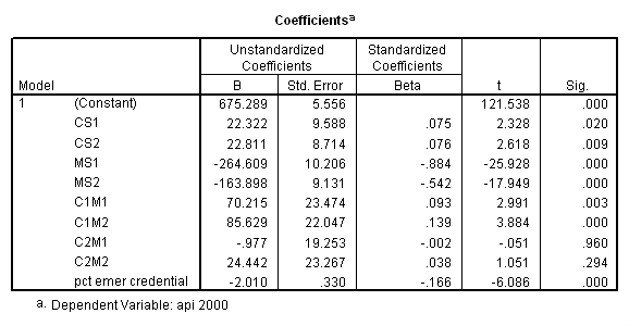
Now we illustrate how to get the same adjusted means if you were to to the analysis via the REGRESSION command. First, we need to create all the necessary dummy variables for the categorical variables. The choice of coding schemes does not matter for the purpose of obtaining the adjusted means. We choose simple coding scheme for both mealcat and collcat below. Regression analysis is done using these dummy variables afterwards.
recode mealcat (1=-.33333)  (2=-.33333)  (3=.66667)  into ms1.
recode mealcat (1= -.33333) (2=.66667)  (3=-.33333)  into ms2.

recode collcat (1=-.33333)  (2=-.33333)  (3=.66667)  into cs1 .
recode collcat (1=-.33333)  (2=.66667)  (3=-.33333)  into cs2 .

compute c1m1 = cs1*ms1.
compute c2m1 = cs2*ms1.
compute c1m2 = cs1*ms2.
compute c2m2 = cs2*ms2.
execute.
regression
/dependent api00
/method=enter cs1 cs2 ms1 ms2 c1m1 c1m2 c2m1 c2m2 emer.
To create the adjusted means we wish to assume that all of the schools are at the average on the variable emer. Let us first find out the mean for emer.
descriptives
  variable=emer
  /statistics=mean.
Now we create yhat as the predicted value based on the regression equation setting emer at its mean. Since the value of emer is set to the mean of emer, this will be the predicted value assuming that all schools are at the average for emer.
compute yhat = 675.289 + 22.322*cs1 + 22.811*cs2
                                    - 264.609*ms1 - 163.898*ms2
                                    + 70.215*c1m1 + 85.629*c1m2
                                    - .977*c2m1 + 24.442*c2m2 - 2.01*12.66.
execute.
Now, we can look at the average of yhat broken down by collcat and mealcat, which you can see corresponds to the adjusted means that we found with glm command above.
means predy  by collcat by mealcat
/cells = mean count.
6.7 More Details on Meaning of the Coefficients
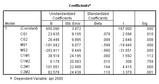
So far we have discussed a variety of techniques that you can use to help interpret interactions of categorical variables in regression, but we have not gone into a great detail about the meaning of the coefficients in these analyses. Let’s consider this further. Consider the analysis below using collcat and mealcat, using simple contrasts on both of these variables. The reference group for both variables will be group 1.
recode mealcat (1= -.33333) (2=.66667)  (3=-.33333)  into ms1.
recode mealcat (1=-.33333)  (2=-.33333)  (3=.66667)  into ms2.

recode collcat (1=-.33333)  (2=.66667)  (3=-.33333) into  cs1 .
recode collcat (1=-.33333)  (2=-.33333)  (3=.66667)  into cs2 .

compute c1m1 = cs1*ms1.
compute c2m1 = cs2*ms1.
compute c1m2 = cs1*ms2.
compute c2m2 = cs2*ms2.
execute.

regression
/dependent api00
/method=enter cs1 cs2 ms1 ms2 c1m1 c1m2 c2m1 c2m2
/save pred(yht1).
We can produce the adjusted means as shown below. These will be useful for interpreting the meaning of the coefficients.
means yht1  by collcat by mealcat
/cells = mean count.
Let’s consider the meaning of the coefficient for cs1. The coding for this variable compares group 2 vs. group 1, hence this coefficient corresponds to mean(collcat = 2) – mean(collcat = 1). Note that these are the unweighted means, so we compute the mean for collcat = 2 as the mean of the 3 cells corresponding to collcat = 2, i.e. (825.651+636.605+508.833)/3 . If we compare the result below to the coefficient for cs1 we see that they are the same,
(825.651+636.605+508.833)/3 – (816.914+589.35+493.919)/3 = 23.635333.
Likewise, the coefficient for cs2 is mean(collcat = 3) – mean(collcat = 1), computed below. The value below corresponds to the coefficient for cs2.
(782.151+655.638+541.733)/3 – (816.914+589.35+493.919)/3 = 26.446333
Likewise, the coefficient for ms1 works out to be mean(mealcat = 2) – mean(mealcat = 1), computed below.
(589.35+636.605+655.638)/3 – (816.914+825.651+782.151)/3 = -181.041.
And the coefficient for ms2 is mean(mealcat = 3) – mean(mealcat = 1), computed below.
(493.919+508.833+541.733)/3 – (816.914+825.651+782.151)/3 = -293.41033
To get the meaning of the coefficients for the interaction terms, let’s write out the regression equation and take a closer look at the coefficients. From the parameter estimates, we have the following linear equation for predicted values:
yhat = 650.090 + 23.635*cs1   + 26.446*cs2
               - 181.042*ms1  - 293.412*ms2
               + 38.518*cs1*ms1  + 6.178*cs1*ms2
               + 101.051*cs2*ms1 + 82.578*cs2*ms2.
Because of the simple coding scheme we use for both variables, we have from the above equation,
yhat(collcat = 2) – yhat(collcat = 1) = 23.635 + 38.518*ms1 + 6.178*ms2.
One way to think about this equation is that for any level of mealcat comparing group 2 vs. group 1 on collcat only involves cs1. It then follows that the coefficient for c1m1 is to compare the difference of group 2 vs. 1 on collcat when mealcat is 2 with the difference of group 2 vs. 1 on collcat when mealcat is 1. In other words, c1m1 is
[cell(2,2)-cell(1,2)] – [cell(2,1)-cell(1,1)].
Plugging all the corresponding cell means to the above formula, we get
(636.6047 – 589.3500) – (825.6512 – 816.9143) = 38.5175,
which is the coefficient for c1m1. Using the same argument, we can have the following
c1m1 : [cell(2,2)-cell(1,2)] – [cell(2,1)-cell(1,1)],
c1m2 : [cell(2,3)-cell(1,3)] – [cell(2,1)-cell(1,1)],
c2m1 : [cell(3,2)-cell(1,2)] – [cell(3,1)-cell(1,1)],
c2m2 : [cell(3,3)-cell(1,3)] – [cell(3,1)-cell(1,1)].
We can go through the same process to verify the meaning of the coefficients for the other 3 interaction terms. We verify that c1m2 is 6.1775.
(508.8333 – 493.9189) – (825.6512 – 816.9143) = 6.1775.
We also verify that c2m1 is 101.051.
(655.6377 – 589.3500) – (782.1509 – 816.9143) = 101.0511.
Last we verify that c2m2 is 82.5778.
( 541.7333 – 493.9189) – ( 782.1509 – 816.9143) = 82.5778.
6.8 Simple Effects via Dummy Coding vs. Effect Coding
We have used in this chapter different types of coding schemes. You may wonder why we have gone to the effort of creating and testing these effects instead of just using dummy coding and what is the difference between different coding schemes and how to choose them. In this section, let’s compare how to get simple effects using the effect coding to how we would get simple effects using dummy coding. We hope to show that it is much easier to use effect coding so that the interpretation of the coefficients is much more intuitive.
6.8.1 Example 1. Simple effects of yr_rnd at levels of mealcat
Let’s use an example from Chapter 3 (section 3.5). In that example we looked at and analysis using mealcat and yr_rnd and the interaction of these two variables. First, we look at how to do a simple effects analysis looking at the simple effects of yr_rnd at each level of mealcat using effect coding. To make our results correspond to those from Chapter 3, we will make category 3 of mealcat the reference category.
recode mealcat (1= .66667)  (2=-.33333)  (3=-.33333)  into ms1.
recode mealcat (1=-.33333)  (2=.66667)  (3=-.33333)  into  ms2.

recode yr_rnd (0=-.5)  (1=.5)  into  yr1.

compute ym1 = 0.
compute ym2 = 0.
compute ym3 = 0.

 if ( mealcat = 1)  ym1 = yr1.
 if ( mealcat = 2)  ym2 = yr1.
 if ( mealcat = 3)  ym3 = yr1.

regression
/dependent api00
/method=enter  ms1 ms2 ym1 ym2 ym3.
Now we can obtain the simple effect of yr_rnd at mealcat = 1 by inspecting the coefficient for ym1, the simple effect of yr_rnd at mealcat = 2 by inspecting the coefficient for ym2 and the simple effect of yr_rnd at mealcat = 3 by inspecting the coefficient for ym3.
Now let’s perform the same analysis using dummy coding. Again, we will explicitly make the 3rd category for mealcat to be the omitted category.
recode mealcat (1= 1)  (2=0)  (3=0)  into md1.
recode mealcat (1=0)  (2=1)  (3=0)  into  md2.

compute ymd1 = yr_rnd*md1.
compute ymd2 = yr_rnd*md2.

regression
/dependent api00
/method=enter  yr_rnd md1 md2 ymd1 ymd2.
In order to form a test of simple main effects we need to make a table like the one shown below that relates the cell means to the coefficients in the regression. Please see Chapter 3, section 3.5 for information on how this table was constructed.
            mealcat=1           mealcat=2         mealcat=3
            -------------------------------------------------
  yr_rnd=0   const               const             const
             + md1               + md2
            -------------------------------------------------
  yr_rnd=1  const               const             const
            + yr_rnd            + yr_rnd          + yr_rnd
            + md1               + md2
            + ymd1              + ymd2
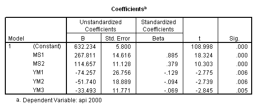
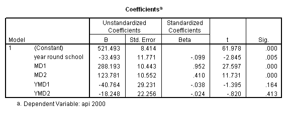
Let’s start by looking at how to get the simple effect of yr_rnd when mealcat is 3. Looking at the table above, we can see that we would want to compare const with const + yr_rnd, , which is the same as testing the coefficient for yr_rnd is zero. This is a single parameter test and is shown in the output above. The t-value is -2.846 and the p-value is .005.
Note that the coefficient for yr_rnd corresponds to the test of the effect of yr_rnd when all other variables are set to 0 (the reference category), i.e. when mealcat is set to the reference category. You may be tempted to interpret the coefficient for yr_rnd as the overall difference between year round schools and non-year round schools, but in this example we see that it really corresponds to the simple effect of yr_rnd. When using dummy coding people commonly misinterpret the lower order effects to refer to overall effects rather than simple effects.
Now let’s look at the simple effect of yr_rnd when mealcat=1. Looking at the table above we see that this involves the comparison of the coefficients for yr_rnd=1 vs. yr_rnd=0 when mealcat=1, i.e. comparing const + yr_rnd +md1 + ymd1 vs. const + md1. Removing the terms that drop out we see that to test the simple effect of yr_rnd when mealcat = 1 is the same to test yr_rnd + ymd1 = 0. This can NOT be done in SPSS through the test command of REGRESSION. We have to use ANOVA type of command to perform the test.
These examples illustrate that it is more complicated to form simple effects when using dummy coding, and also that the interpretation of lower order effects when using dummy coding may not have the meaning that you would expect.
6.8.2 Example 2. Simple effects of mealcat at levels of yr_rnd
Example 1 looked at simple effects for yr_rnd, a variable with only 2 levels and it showed that the REGRESSION procedure in SPSS is very limited on its test subcommand. In this example, let’s consider the simple effects of mealcat at each level of yr_rnd. Because mealcat has more than 2 levels, we will see what is required for doing tests of simple effects for variables with more than 2 levels. We will use procedure GLM to perform all the necessary tests to test the simple effects.
First, let’s show how to get these simple effects using the MANOVA.
manova api00 by yr_rnd(0,1) mealcat(1,3)
  /error =  w
  /design = yr_rnd
                mealcat within yr_rnd(1)
                mealcat within yr_rnd(2).
* * * * * * A n a l y s i s   o f   V a r i a n c e * * * * * *

       400 cases accepted.
         0 cases rejected because of out-of-range factor values.
         0 cases rejected because of missing data.
         6 non-empty cells.

         1 design will be processed.

* * * * * * A n a l y s i s   o f   V a r i a n c e -- design   1 * * * * * *

 Tests of Significance for API00 using UNIQUE sums of squares
 Source of Variation          SS      DF        MS         F  Sig of F

 WITHIN CELLS         1868944.18     394   4743.51
 YR_RND                 99617.37       1  99617.37     21.00      .000
 MEALCAT WITHIN YR_RN 3903569.80       2 1951784.9    411.46      .000
 D(1)
 MEALCAT WITHIN YR_RN  476157.45       2 238078.73     50.19      .000
 D(2)

 (Model)              6204727.82       5 1240945.6    261.61      .000
 (Total)              8073672.00     399  20234.77

 R-Squared =           .769
 Adjusted R-Squared =  .766
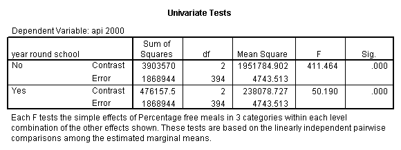
The simple effect of mealcat when yr_rnd = 0 is shown in the above ANOVA table with F-value 411.46 and p-value .000. The simple effect of mealcat when yr_rnd = 1 is significant with F-value 50.19. Now we show how to get the same analysis using GLM.
glm api00 by yr_rnd mealcat
/emmeans tables(yr_rnd*mealcat) compare(mealcat).

