Version info: Code for this page was tested in Stata 12.
Zero-truncated poisson regression is used to model count data for which the value zero cannot occur.
Please Note: The purpose of this page is to show how to use various data analysis commands. It does not cover all aspects of the research process which researchers are expected to do. In particular, it does not cover data cleaning and verification, verification of assumptions, model diagnostics and potential follow-up analyses.
Examples of zero-truncated Poisson regression
Example 1.
A study of length of hospital stay, in days, as a function of age, kind of health insurance and whether or not the patient died while in the hospital. Length of hospital stay is recorded as a minimum of at least one day.
Example 2.
A study of the number of journal articles published by tenured faculty as a function of discipline (fine arts, science, social science, humanities, medical, etc). To get tenure faculty must publish, therefore, there are no tenured faculty with zero publications.
Example 3.
A study by the county traffic court on the number of tickets received by teenagers as predicted by school performance, amount of driver training and gender. Only individuals who have received at least one citation are in the traffic court files.
Description of the data
Let’s pursue Example 1 from above.
We have a hypothetical data file, ztp.dta with 1,493 observations.
The length of hospital stay variable is stay
Let’s look at the data.
use https://stats.idre.ucla.edu/stat/data/ztp, clear

summarize stay

    Variable |       Obs        Mean    Std. Dev.       Min        Max
-------------+--------------------------------------------------------
        stay |      1493    9.728734    8.132908          1         74

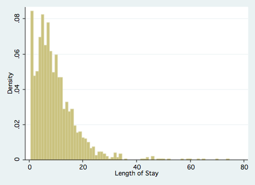
histogram stay, discrete


tab1 age hmo died

-> tabulation of age

  Age Group |      Freq.     Percent        Cum.
------------+-----------------------------------
          1 |          6        0.40        0.40
          2 |         60        4.02        4.42
          3 |        163       10.92       15.34
          4 |        291       19.49       34.83
          5 |        317       21.23       56.06
          6 |        327       21.90       77.96
          7 |        190       12.73       90.69
          8 |         93        6.23       96.92
          9 |         46        3.08      100.00
------------+-----------------------------------
      Total |      1,493      100.00

-> tabulation of hmo

        hmo |      Freq.     Percent        Cum.
------------+-----------------------------------
          0 |      1,254       83.99       83.99
          1 |        239       16.01      100.00
------------+-----------------------------------
      Total |      1,493      100.00

-> tabulation of died

       died |      Freq.     Percent        Cum.
------------+-----------------------------------
          0 |        981       65.71       65.71
          1 |        512       34.29      100.00
------------+-----------------------------------
      Total |      1,493      100.00
Analysis methods you might consider
Below is a list of some analysis methods you may have encountered. Some of the methods listed are quite reasonable while others have either fallen out of favor or have limitations.
- Zero-truncated Poisson Regression – The focus of this web page.
- Zero-truncated Negative Binomial Regression – If you have overdispersion in addition to zero truncation. See the Data Analysis Example for ztnb.
- Poisson Regression – Ordinary Poisson regression will have difficulty with zero-truncated data. It will try to predict zero counts even though there are no zero values.
- Negative Binomial Regression – Ordinary Negative Binomial regression will have difficulty with zero-truncated data. It will try to predict zero counts even though there are no zero values.
- OLS Regression – You could try to analyze these data using OLS regression. However, count data are highly non-normal and are not well estimated by OLS regression.
Zero-truncated Poisson regression
You can use the tpoisson command for zero-truncated poisson regression. The tpoisson command will analyze models that are left truncated on any value not just zero. Additionally, since Cameron and Trivedi (2009) recommend robust standard errors for poisson models we will include the vce(robust) option.
tpoisson stay age i.hmo i.died, ll(0) vce(robust)

Iteration 0:   log pseudolikelihood = -6908.7992
Iteration 1:   log pseudolikelihood = -6908.7991

Truncated Poisson regression                      Number of obs   =       1493
Truncation point: 0                               Wald chi2(3)    =      25.65
                                                  Prob > chi2     =     0.0000
Log pseudolikelihood = -6908.7991                 Pseudo R2       =     0.0129

------------------------------------------------------------------------------
             |               Robust
        stay |      Coef.   Std. Err.      z    P>|z|     [95% Conf. Interval]
-------------+----------------------------------------------------------------
         age |   -.014442   .0121867    -1.19   0.236    -.0383276    .0094436
       1.hmo |  -.1359033   .0520484    -2.61   0.009    -.2379163   -.0338902
      1.died |  -.2037709   .0491608    -4.14   0.000    -.3001242   -.1074175
       _cons |   2.435808   .0708745    34.37   0.000     2.296897     2.57472
------------------------------------------------------------------------------
The output looks very much like the output from an OLS regression:
- It begins with the iteration log giving the values of the log pseudolikelihoods starting with a model that has no predictors.
- The last value in the log (-6908.7991) is the final value of the log pseudolikelihood for the full model and is repeated below.
- Next comes the header information. On the right-hand side the number of observations used (1493) is given along with the likelihood ratio chi-squared with three degrees of freedom for the full model, followed by the p-value for the chi-square. The model, as a whole, is statistically significant.
- The header also includes a pseudo-R2 which is very low in this example (0.0129).
- Below the header you will find the zero-truncated poisson coefficients for each of the variables along with standard errors, z-scores, p-values and 95% confidence intervals for each coefficient.
Looking through the results we see the following:
- The value of the coefficient for age, -.014442, suggests that the log count of stay decreases by .014442 for each year increase in age. This coefficient is not statistically significant.
- The coefficient for hmo, -.1359, is significant and indicates that the log count of stay for HMO patient is .1359 less than for non-HMO patients.
- The log count of stay for patients who died while in the hospital was .20377 less than those patients who did not die.
- Finally, the value of the constant (_cons), 2.4358 is log count of the stay when all of the predictors equal zero.
We can also use the margins command to help understand our model.
For example we can find the expected number of days spent at the hospital across age groups for the two hmo statuses and for the two died statuses.
margins hmo, at(age=(1(1)9)) vsquish

Predictive margins                                Number of obs   =       1493
Model VCE    : Robust

Expression   : Predicted number of events, predict()
1._at        : age             =           1
2._at        : age             =           2
3._at        : age             =           3
4._at        : age             =           4
5._at        : age             =           5
6._at        : age             =           6
7._at        : age             =           7
8._at        : age             =           8
9._at        : age             =           9

------------------------------------------------------------------------------
             |            Delta-method
             |     Margin   Std. Err.      z    P>|z|     [95% Conf. Interval]
-------------+----------------------------------------------------------------
     _at#hmo |
        1 0  |    10.5493   .6310057    16.72   0.000     9.312549    11.78605
        1 1  |   9.208768   .6261728    14.71   0.000     7.981491    10.43604
        2 0  |   10.39804   .5078432    20.47   0.000     9.402685    11.39339
        2 1  |    9.07673    .541332    16.77   0.000     8.015739    10.13772
        3 0  |   10.24895   .3956085    25.91   0.000     9.473572    11.02433
        3 1  |   8.946586   .4723194    18.94   0.000     8.020857    9.872315
        4 0  |     10.102   .3016365    33.49   0.000     9.510801    10.69319
        4 1  |   8.818307   .4242343    20.79   0.000     7.986823    9.649792
        5 0  |   9.957153   .2419017    41.16   0.000     9.483034    10.43127
        5 1  |   8.691868   .4019681    21.62   0.000     7.904025    9.479712
        6 0  |   9.814385   .2375591    41.31   0.000     9.348778    10.27999
        6 1  |   8.567242   .4072901    21.03   0.000     7.768969    9.365516
        7 0  |   9.673664   .2867397    33.74   0.000     9.111665    10.23566
        7 1  |   8.444403   .4370317    19.32   0.000     7.587837     9.30097
        8 0  |   9.534961   .3653709    26.10   0.000     8.818847    10.25107
        8 1  |   8.323325   .4848934    17.17   0.000     7.372952    9.273699
        9 0  |   9.398246   .4560941    20.61   0.000     8.504318    10.29217
        9 1  |   8.203984   .5445834    15.06   0.000      7.13662    9.271347
------------------------------------------------------------------------------
We can see that the number of days spent tends to decrease as we move up age groups (the left column under _at#hmo) and that patients enrolled in an hmo (the right column under _at#hmo) tend to spend fewer days at the hospital as well than those not in hmos. For example, we expect that a non-hmo patient in age group 1 to stay for 10.5493 days whereas an hmo patient in age group 1 is expected to stay 9.2088 days. We can plot the number of days predicted by age group and hmo status using the marginsplot command.
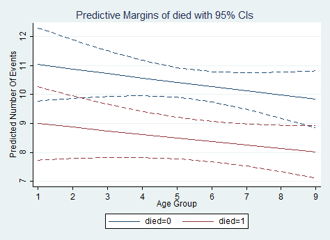
marginsplot, recast(line) recastci(rline) ciopts(lpattern(dash))margins died, at(age=(1(1)9)) vsquish Predictive margins Number of obs = 1493 Model VCE : Robust Expression : Predicted number of events, predict() 1._at : age = 1 2._at : age = 2 3._at : age = 3 4._at : age = 4 5._at : age = 5 6._at : age = 6 7._at : age = 7 8._at : age = 8 9._at : age = 9 ------------------------------------------------------------------------------ | Delta-method | Margin Std. Err. z P>|z| [95% Conf. Interval] -------------+---------------------------------------------------------------- _at#died | 1 0 | 11.03216 .6419426 17.19 0.000 9.773975 12.29034 1 1 | 8.998372 .6434904 13.98 0.000 7.737154 10.25959 2 0 | 10.87398 .5155445 21.09 0.000 9.863529 11.88443 2 1 | 8.869352 .5506018 16.11 0.000 7.790192 9.948511 3 0 | 10.71806 .4019963 26.66 0.000 9.930166 11.50596 3 1 | 8.742181 .4700277 18.60 0.000 7.820943 9.663418 4 0 | 10.56439 .3102963 34.05 0.000 9.956216 11.17256 4 1 | 8.616833 .4064251 21.20 0.000 7.820255 9.413412 5 0 | 10.41291 .2583831 40.30 0.000 9.906489 10.91933 5 1 | 8.493283 .3658669 23.21 0.000 7.776197 9.210369 6 0 | 10.26361 .2648261 38.76 0.000 9.744559 10.78266 6 1 | 8.371504 .3535566 23.68 0.000 7.678546 9.064462 7 0 | 10.11645 .321958 31.42 0.000 9.48542 10.74747 7 1 | 8.251472 .3698185 22.31 0.000 7.526641 8.976303 8 0 | 9.971394 .4058928 24.57 0.000 9.175859 10.76693 8 1 | 8.13316 .4091532 19.88 0.000 7.331234 8.935086 9 0 | 9.828422 .5009702 19.62 0.000 8.846538 10.81031 9 1 | 8.016545 .463983 17.28 0.000 7.107155 8.925935 ------------------------------------------------------------------------------
We can see that the number of days spent tends to decrease as we move up age groups again (the left column under _at#hmo) and that patients died (the right column under _at#hmo) tend to spend fewer days at the hospital than those that did not die (died = 0). For example, we expect that a patient who died in age group 1 to stay for 8.998372 days whereas a patient who lived in age group 1 is expected to stay 11.03216 days. We can plot the number of days predicted by age group and died status using the marginsplot command.
marginsplot, recast(line) recastci(rline) ciopts(lpattern(dash))
The AIC and BIC are useful for model comparisons. You can look at these criteria using the estat ic command.
estat ic

-----------------------------------------------------------------------------
       Model |    Obs    ll(null)   ll(model)     df          AIC         BIC
-------------+---------------------------------------------------------------
           . |   1493   -6999.365   -6908.799      4      13825.6    13846.83
-----------------------------------------------------------------------------
               Note:  N=Obs used in calculating BIC; see [R] BIC note
Things to consider
- Count data often use exposure variable to indicate the number of times the event could have happened. You can incorporate exposure into your model by using the exposure() option.
- It is not recommended that zero-truncated poisson models be applied to small samples. What constitutes a small sample does not seem to be clearly defined in the literature.
- Pseudo-R-squared values differ from OLS R-squareds, please see FAQ: What are pseudo R-squareds? for a discussion on this issue.
See Also
References
- Cameron, A. Colin and Trivedi, P.K. (2009) Microeconometrics using stata. College Station, TX: Stata Press.
- Long, J. Scott, & Freese, Jeremy (2006). Regression Models for Categorical Dependent Variables Using Stata (Second Edition). College Station, TX: Stata Press.
- Long, J. Scott (1997). Regression Models for Categorical and Limited Dependent Variables. Thousand Oaks, CA: Sage Publications.
