
The purpose of this workshop is to explore some issues in the analysis of
survey data using StataNow 18.5. Before we begin, you will want to be sure that
your copy of Stata is up-to-date. To do this, please type
update all
in the Stata command window and follow any instructions given. These
updates include not only fixes to known bugs, but also add some new features
that may be useful.
Before we begin looking at examples in Stata,
we will quickly review some basic issues and concepts in survey data analysis.
NOTE: Most of the commands in this seminar will work with Stata versions 12-17.
You can download the PowerPoint slides and the answers to the questions in the PowerPoint slides.
Why do we need survey data analysis software?
Regular procedures in statistical software (that is not designed for survey
data) analyzes data as if the data were collected using simple random sampling.
For experimental and quasi-experimental designs, this is exactly what we want.
However, very few surveys use a simple random sample to collect data.
Not only is it nearly impossible to do so, but it is not as efficient (either
financially and statistically) as other sampling methods. When any
sampling method other than simple random sampling is used, we usually need to use survey
data analysis software to take into account the differences between the design
that was used to collect the data and simple random sampling. This is because the sampling design affects
both the calculation of the
point estimates and the standard errors of those estimates. If you ignore the sampling design, e.g.,
if you assume simple random sampling when another type of sampling design was
used, both the point estimates and their standard errors will likely be
calculated incorrectly. The sampling weight will affect the calculation of
the point estimate, and the stratification and/or clustering will affect the
calculation of the standard errors. Ignoring the clustering will likely
lead to standard errors that are underestimated, possibly leading to
results that seem to be statistically significant, when in fact, they are not.
The difference in point estimates and standard errors obtained using non-survey
software and survey software with the design properly specified will vary from
data set to data set, and even between analyses using the same data set.
While it may be possible to get reasonably accurate results using non-survey
software, there is no practical way to know beforehand how far off the results
from non-survey software will be.
Sampling designs
Most people do not conduct their own surveys. Rather, they
use survey data that some agency or company collected and made available to the
public. The documentation must be read carefully to find out what kind of
sampling design was used to collect the data. This is very important
because many of the estimates and standard errors are calculated differently for
the different sampling designs. Hence, if you mis-specify the sampling
design, the point estimates and standard errors will likely be wrong.
Below are some common features of many sampling designs.
Sampling weights: There are several types of weights that
can be associated with a survey. Perhaps the most common is the sampling weight.
A sampling weight is a probability weight that has had one or more adjustments
made to it. Both a sampling weight and a probability weight are used to weight the sample back to the population from which the sample
was drawn. By definition, a probability weight is the inverse of the probability of being included in the
sample due to the sampling design (except for a certainty PSU, see below).
The probability weight, called a pweight in Stata, is calculated as N/n, where N = the number of elements in the
population and n = the number of elements in the sample. For example, if a population has 10
elements and 3 are sampled at random with replacement, then the probability weight would be
10/3 = 3.33. In a two-stage design, the probability weight is calculated as f1f2,
which means that the inverse of the sampling fraction for the first stage is
multiplied by the inverse of the sampling fraction for the second stage.
Under many sampling plans, the sum of the probability weights will equal the population total.
While many textbooks will end their discussion of probability weights here, this
definition does not fully describe the sampling weights that are included with actual
survey data sets. Rather, the sampling weight, which is sometimes called a “final weight,” starts with the
inverse of the sampling fraction, but then incorporates several other values,
such as corrections for unit non-response, errors in the sampling frame
(sometimes called non-coverage), calibration and trimming. Because these
other values are included in the probability weight that is included with the data
set, it is often inadvisable to modify the sampling weights, such as trying to
standardize them for a particular variable, e.g., age.
Strata: Stratification is a method of breaking up the
population into different groups, often by demographic variables such as gender,
race or SES. Each element in the population must belong to one, and only
one, strata. Once the strata have been defined, samples are taken from each
stratum as if it were independent of all of the other strata. For example,
if a sample is to be stratified on gender, men and women would be sampled
independently of one another. This means that the probability weights for men will
likely be different from the probability weights for the women. In most cases, you
need to have two or more PSUs in each stratum. The purpose of
stratification is to reduce the standard error of the estimates, and stratification works most
effectively when the variance of the dependent variable is smaller within the
strata than in the sample as a whole.
PSU: This is the primary sampling unit.
This is the first unit that is sampled in the design. For example, school
districts from California may be sampled and then schools within districts may
be sampled. The school district would be the PSU. If states from the US were sampled, and then school districts from within each
state, and then schools from within each district, then states would be the PSU.
One does not need to use the same sampling method at all levels of sampling.
For example, probability-proportional-to-size sampling may be used at
level 1 (to select states), while cluster sampling is used at level 2
(to select school districts). In the case of a simple random sample, the
PSUs and the elementary units are the same. In general, accounting for the
clustering in the data (i.e., using the PSUs), will increase the standard errors
of the point estimates. Conversely, ignoring the PSUs will tend to yield
standard errors that are too small, leading to false positives when doing
significance tests.
FPC: This is the finite population correction.
This is used when the sampling fraction (the number of elements or respondents
sampled relative to the population) becomes large. The FPC is used in the
calculation of the standard error of the estimate. If the value of the FPC
is close to 1, it will have little impact and can be safely ignored. In
some survey data analysis programs, such as SUDAAN, this information will be
needed if you specify that the data were collected without replacement
(see below for a definition of “without replacement”). The
formula for calculating the FPC is ((N-n)/(N-1))1/2, where N is the
number of elements in the population and n is the number of elements in the
sample. To see the impact of the FPC for
samples of various proportions, suppose that you had
a population of 10,000 elements.
Sample size (n)    FPC
1                1.0000
10                .9995
100               .9950
500               .9747
1000              .9487
5000              .7071
9000              .3162
Replicate weights: Replicate weights are a series of weight
variables that are used to correct the standard errors for the sampling plan.
They serve the same function as the PSU and strata variables (which are used a Taylor series
linearization) to correct the standard errors of the estimates for the sampling
design. Many public use data sets are now being released with
replicate weights instead of PSUs and strata in an effort to more securely
protect the identity of the respondents. In theory, the same standard
errors will be obtained using either the PSU and strata or the replicate
weights. There are different ways of creating replicate weights; the
method used is determined by the sampling plan. The most common are
balanced repeated and jackknife replicate weights. You will need to read
the documentation for the survey data set carefully to learn what type of
replicate weight is included in the data set; specifying the wrong type of
replicate weight will likely lead to incorrect standard errors. For more
information on replicate weights, please see Stata Library: Replicate Weights and Appendix D of the
WesVar Manual by Westat, Inc. Several statistical packages, including Stata, SAS, R, Mplus, SUDAAN and WesVar, allow the use of replicate weights.
Consequences of not using the design elements
Sampling design elements include the sampling weights, post-stratification
weights (if provided), PSUs, strata, and replicate weights. Rarely are all
of these elements included in a single public-use data set. However,
ignoring the design elements that are included can often lead to inaccurate
point estimates and/or inaccurate standard errors.
Sampling with and without replacement
Most samples collected in the real world are collected “without
replacement”. This means that once a respondent has been selected to be in
the sample and has participated in the survey, that particular respondent cannot
be selected again to be in the sample. Many of the calculations change
depending on if
a sample is collected with or without replacement. Hence, programs like
SUDAAN request that you specify if a survey sampling design was implemented with
our without replacement, and an FPC is used if sampling without replacement is
used, even if the value of the FPC is very close to one.
Examples
For the examples in this workshop, we will use the data set from NHANES (the National Health and Nutrition Examination Survey)
that comes with Stata.
Reading the documentation
The first step in analyzing any survey data set is to read the documentation.
With many of the public use data sets, the documentation can be quite extensive
and sometimes even intimidating. Instead of trying to read the
documentation “cover to cover”, there are some parts you will want to focus on.
First, read the Introduction. This is usually an “easy read” and will
orient you to the survey. There is usually a section or chapter called
something like
“Sample Design and Analysis Guidelines”, “Variance Estimation”, etc. This
is the part that tells you about the design elements included with the survey
and how to use them. Some even give example code. If multiple
sampling weights have been included in the data set, there will be some
instruction about when to use which one. If there is a section or chapter
on missing data or imputation, please read that. This will tell you how
missing data were handled. You should also read any documentation
regarding the specific variables that you intend to use. As we will see
little later on, we will need to look at the documentation to get the value
labels for the variables. This is especially important because some of the
values are actually missing data codes, and you need to do something so that
Stata doesn’t treat those as valid values (or you will get some very
“interesting” means, totals, etc.).
Getting NHANES data into Stata
For the examples in this workshop, we will be using a version of the NHANES II dataset that comes with Stata. However, for real analyses, you need to download data from the NHANES website.
Checking the sampling weight
The svyset command
Before we can start our analyses, we need to issue the
svyset command. The svyset command tells Stata about the design
elements in the survey. Once this command has been issued, all you need to
do for your analyses is use the svy: prefix before each command.
Because the 2011-2012 NHANES data were released with a sampling weight (wtint2yr), a PSU
variable (sdmvpsu) and a strata variable (sdmvstra), we will use these our svyset command. The svyset command looks like this:
use https://www.stata-press.com/data/r18/nhanes2f, clear
sum finalwgt

    Variable |        Obs        Mean    Std. dev.       Min        Max
-------------+---------------------------------------------------------
    finalwgt |     10,337    11320.85    7304.457       2000      79634

count if finalwgt == .
  0

count if stratid == .
  0

count if psuid == .
  0

svyset psuid [pweight=finalwgt], strata(stratid) singleunit(centered)
Sampling weights: finalwgt VCE: linearized Single unit: centered Strata 1: stratid Sampling unit 1: psuid FPC 1:
The singleunit option was added in Stata 10. This option allows for
different ways of handling a single PSU in a stratum. There are usually two or more PSUs in each stratum. If there is only one PSU in stratum, due to missing data or a subpopulation specification, for example, the variance cannot be estimated in that stratum. If you use the
default option, missing, then you will get no standard errors when Stata
encounters a single PSU in a stratum. There are three other options.
One is certainty, meaning that the singleton PSUs be treated as certainty
PSUs; certainty PSUs are PSUs that were selected into the sample with a
probability of 1 (in other words, these PSUs were certain to be in the sample)
and do not contribute to the standard error. The scaled option
gives a scaled version of the certainty option. The scaling factor comes
from using the average of the variances from the strata with multiple sampling
units for each stratum with one PSU. The centered option centers
strata with one sampling unit at the grand mean instead of the stratum mean.
Now that we have issued the svyset command, we can use the svydescribe
command to get information on the strata and PSUs. It is a good idea to use this command to learn about the strata and PSUs in the dataset.
svydescribeSurvey: Describing stage 1 sampling units Sampling weights: finalwgt VCE: linearized Single unit: centered Strata 1: stratid Sampling unit 1: psuid FPC 1: Number of obs per unit Stratum # units # obs Min Mean Max ---------------------------------------------------------- 1 2 380 165 190.0 215 2 2 185 67 92.5 118 3 2 348 149 174.0 199 4 2 460 229 230.0 231 5 2 252 105 126.0 147 6 2 298 131 149.0 167 7 2 476 206 238.0 270 8 2 337 158 168.5 179 9 2 243 100 121.5 143 10 2 262 119 131.0 143 11 2 275 120 137.5 155 12 2 314 144 157.0 170 13 2 342 154 171.0 188 14 2 405 200 202.5 205 15 2 380 189 190.0 191 16 2 336 159 168.0 177 17 2 393 180 196.5 213 18 2 359 144 179.5 215 20 2 283 125 141.5 158 21 2 213 102 106.5 111 22 2 301 128 150.5 173 23 2 340 158 170.0 182 24 2 434 202 217.0 232 25 2 254 115 127.0 139 26 2 261 129 130.5 132 27 2 283 139 141.5 144 28 2 298 135 149.0 163 29 2 502 215 251.0 287 30 2 365 166 182.5 199 31 2 308 143 154.0 165 32 2 450 211 225.0 239 ---------------------------------------------------------- 31 62 10,337 67 166.7 287
The output above tells us that there are 31 strata with two PSUs in
each. There are 62 PSUs. There are a different number of
observations in each PSU and in each strata. There are a minimum of 67
observations, a maximum of 287 observations and an average of 166.7 observations
in the PSUs. The design degrees of freedom is calculated as the number of strata minus the number of PSUs. For this data set, that is 62-31 = 31.
Descriptive statistics
We will start by calculating some descriptive statistics of some of the
continuous variables. We can use the svy: mean command to get the
mean of continuous variables, and we can follow that command with the estat
sd command to get the standard deviation or variance of the variable. The var option on the estat sd command can be used to get the variance.
svy: mean age
(running mean on estimation sample)

Survey: Mean estimation

Number of strata = 31            Number of obs   =      10,337
Number of PSUs   = 62            Population size = 117,023,659
                                 Design df       =          31

--------------------------------------------------------------
             |             Linearized
             |       Mean   std. err.     [95% conf. interval]
-------------+------------------------------------------------
         age |   42.23732   .3034412      41.61844    42.85619
--------------------------------------------------------------

estat sd

-------------------------------------
             |       Mean   Std. dev.
-------------+-----------------------
         age |   42.23732    15.50095
-------------------------------------

estat sd, var

-------------------------------------
             |       Mean    Variance
-------------+-----------------------
         age |   42.23732    240.2795
-------------------------------------

svy: mean copper
(running mean on estimation sample)

Survey: Mean estimation

Number of strata = 31            Number of obs   =       9,118
Number of PSUs   = 62            Population size = 103,505,700
                                 Design df       =          31

--------------------------------------------------------------
             |             Linearized
             |       Mean   std. err.     [95% conf. interval]
-------------+------------------------------------------------
      copper |   124.7232   .6657517      123.3654     126.081
--------------------------------------------------------------

svy: mean hct // hemocrit
(running mean on estimation sample)

Survey: Mean estimation

Number of strata = 31            Number of obs   =      10,337
Number of PSUs   = 62            Population size = 117,023,659
                                 Design df       =          31

--------------------------------------------------------------
             |             Linearized
             |       Mean   std. err.     [95% conf. interval]
-------------+------------------------------------------------
         hct |   41.98352   .0762331      41.82804      42.139
--------------------------------------------------------------
Notice that a different number of observations were used in each analysis.
This is important, because if you use these three variables in the same call to
svy: mean, you will get different estimates of the means for each of the
variables. This is because copper has
missing values. There are 9118 observations that have valid (AKA non-missing) values for all three variables,
and those are used in the calculations of the means when all of the variables
are used in the same call to svy: mean.
svy: mean age copper hct
(running mean on estimation sample)

Survey: Mean estimation

Number of strata = 31            Number of obs   =       9,118
Number of PSUs   = 62            Population size = 103,505,700
                                 Design df       =          31

--------------------------------------------------------------
             |             Linearized
             |       Mean   std. err.     [95% conf. interval]
-------------+------------------------------------------------
         age |   42.32525   .3239445      41.66457    42.98594
      copper |   124.7232   .6657517      123.3654     126.081
         hct |   41.97078   .0843598      41.79873    42.14283
--------------------------------------------------------------
Let’s get some descriptive statistics a
binary variable such as female.
svy: mean female
(running mean on estimation sample)

Survey: Mean estimation

Number of strata = 31            Number of obs   =      10,337
Number of PSUs   = 62            Population size = 117,023,659
                                 Design df       =          31

--------------------------------------------------------------
             |             Linearized
             |       Mean   std. err.     [95% conf. interval]
-------------+------------------------------------------------
      female |   .5204215    .005773      .5086474    .5321956
--------------------------------------------------------------

estat sd

-------------------------------------
             |       Mean   Std. dev.
-------------+-----------------------
      female |   .5204215     .499607
-------------------------------------
Taking the mean of a variable that is coded 0/1 gives the proportion of 1s.
The output above indicates that approximately 52% of the observations in our
data set are from females.
Of course, the svy: tab command can also be used with binary
variables. The proportion of .5204 matches the .5204215 that we found with
the svy: mean command.
svy: tab female
(running tabulate on estimation sample)

Number of strata = 31                            Number of obs   =      10,337
Number of PSUs   = 62                            Population size = 117,023,659
                                                 Design df       =          31

----------------------
   Female | proportion
----------+-----------
     Male |      .4796
   Female |      .5204
          |
    Total |          1
----------------------
Key: proportion = Cell proportion
Of course, the svy: proportion command can also be used to get
proportions.
svy: proportion female
(running proportion on estimation sample)

Survey: Proportion estimation

Number of strata = 31            Number of obs   =      10,337
Number of PSUs   = 62            Population size = 117,023,659
                                 Design df       =          31

--------------------------------------------------------------
             |             Linearized            Logit
             | Proportion   std. err.     [95% conf. interval]
-------------+------------------------------------------------
      female |
       Male  |   .4795785    .005773      .4678179    .4913618
     Female  |   .5204215    .005773      .5086382    .5321821
--------------------------------------------------------------
Using the estat post-estimation command after the svy: mean command also allows
you to get the design effects, misspecification effects, unweighted and weighted
sample sizes, or the coefficient of variation.
The Deff and the Deft are types of design
effects, which tell you about the efficiency of your sample. The Deff is a
ratio of two variances. In the numerator we have the variance estimate
from the current sample (including all of its design elements), and in the
denominator we have the variance from a hypothetical sample of the same size
drawn as an SRS. In other words, the Deff tells you how efficient your
sample is compared to an SRS of equal size. If the Deff is less than 1,
your sample is more efficient than SRS; usually the Deff is greater than 1.
The Deft is the ratio of two standard error estimates. Again, the
numerator is the standard error estimate from the current sample. The
denominator is a hypothetical SRS (with replacement) standard error from a
sample of the same size as the current sample.
You can also use the meff and the
meft option to get the misspecification effects.
Misspecification effects are a ratio of the variance estimate from the current
analysis to a hypothetical variance estimated from a misspecified model.
Please see the Stata documentation for more details on how these are calculated.
The coefficient of variation is the ratio of the standard error to the mean,
multiplied by 100% (see page 36 of the Stata 18 svy manual). It is an
indication of the variability relative to the mean in the population and is not
affected by the unit of measurement of the variable.
svy: mean age
(running mean on estimation sample)

Survey: Mean estimation

Number of strata = 31            Number of obs   =      10,337
Number of PSUs   = 62            Population size = 117,023,659
                                 Design df       =          31

--------------------------------------------------------------
             |             Linearized
             |       Mean   std. err.     [95% conf. interval]
-------------+------------------------------------------------
         age |   42.23732   .3034412      41.61844    42.85619
--------------------------------------------------------------

estat effects

----------------------------------------------------------
             |             Linearized
             |       Mean   std. err.       DEFF      DEFT
-------------+--------------------------------------------
         age |   42.23732   .3034412      3.9612   1.99028
----------------------------------------------------------

estat effects, deff deft meff meft

------------------------------------------------------------------------------
             |             Linearized
             |       Mean   std. err.       DEFF      DEFT      MEFF      MEFT
-------------+----------------------------------------------------------------
         age |   42.23732   .3034412      3.9612   1.99028     3.211   1.79193
------------------------------------------------------------------------------

estat cv

------------------------------------------------
             |             Linearized
             |       Mean   std. err.     CV (%)
-------------+----------------------------------
         age |   42.23732   .3034412      .71842
------------------------------------------------
display (.3034412/42.23732)*100 .71841963
Graphing with continuous variables
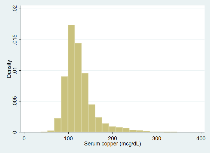
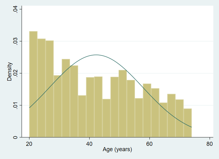
We can also get some descriptive graphs of our variables. For a continuous variable, you may want a histogram. However, the histogram command will only accept a frequency weight, which, by definition, can have only integer values. A suggestion by Heeringa, West and Berglund (2010, pages 121-122) is to simply use the integer part of the sampling weight. We can create a frequency weight from our sampling weight using the generate command with the int function.
gen int_finalwgt = int(finalwgt)
histogram copper [fw = int_finalwgt], bin(20)
We can make box plots and use the sampling weight that is provided in the
data set.
graph box hct [pw = finalwgt]
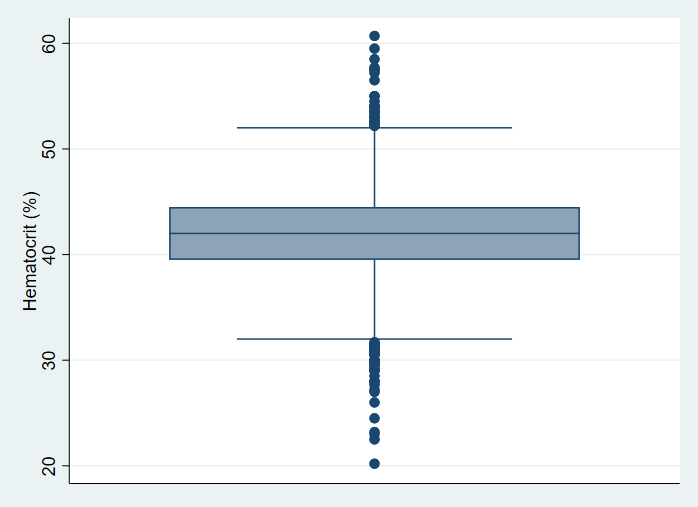
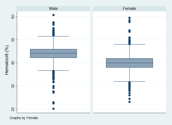
The line in the box plot represents the median, not the mean.
svy, over(female): mean hct
(running mean on estimation sample)

Survey: Mean estimation

Number of strata = 31            Number of obs   =      10,337
Number of PSUs   = 62            Population size = 117,023,659
                                 Design df       =          31

--------------------------------------------------------------
             |             Linearized
             |       Mean   std. err.     [95% conf. interval]
-------------+------------------------------------------------
c.hct@female |
       Male  |   44.21309   .0730382      44.06412    44.36205
     Female  |   39.92893   .0857013      39.75414    40.10372
--------------------------------------------------------------

estat sd

-------------------------------------
        Over |       Mean   Std. dev.
-------------+-----------------------
c.hct@female |
       Male  |   44.21309    2.891824
     Female  |   39.92893     3.02211
-------------------------------------
There is no survey command in Stata that will give us the median, but we can use a “hack” and specify the sampling weight as an analytic weight. (Please see https://www.stata.com/support/faqs/statistics/percentiles-for-survey-data/ for more information.)
bysort female: summarize hct [aw = finalwt], detail

----------------------------------------------------------------------------------------------------------------------------
-> female = Male

                       Hematocrit (%)
-------------------------------------------------------------
      Percentiles      Smallest
 1%           37           20.2
 5%         39.5           22.5
10%         40.7             23       Obs               4,909
25%         42.2           27.2       Sum of wgt.    56122035

50%         44.2                      Mean           44.21309
                        Largest       Std. dev.      2.906201
75%           46           57.2
90%         47.7           57.5       Variance       8.446005
95%         48.7           57.5       Skewness      -.2544314
99%           51           60.7       Kurtosis       5.152102

----------------------------------------------------------------------------------------------------------------------------
-> female = Female

                       Hematocrit (%)
-------------------------------------------------------------
      Percentiles      Smallest
 1%           33           23.2
 5%           35           24.5
10%         36.2             26       Obs               5,428
25%           38             27       Sum of wgt.    60901624

50%           40                      Mean           39.92893
                        Largest       Std. dev.      3.008737
75%           42             54
90%         43.7           57.7       Variance       9.052499
95%           45           58.5       Skewness       .0781784
99%           47           59.5       Kurtosis       4.524747
We can get the ratio of two continuous variables with the svy: ratio command. In this example, we will use copper and hct.
svy: ratio copper hct
(running ratio on estimation sample)

Survey: Ratio estimation

Number of strata = 31            Number of obs   =       9,118
Number of PSUs   = 62            Population size = 103,505,700
                                 Design df       =          31

     _ratio_1: copper/hct

--------------------------------------------------------------
             |             Linearized
             |      Ratio   std. err.     [95% conf. interval]
-------------+------------------------------------------------
    _ratio_1 |   2.971668   .0179592       2.93504    3.008296
--------------------------------------------------------------
What would we do if we wanted to get the ratio of women to men? We would create a new variable (probably called male) and the use the svy: ratio command as before.
gen male = !female
tab female male

           |         male
    Female |         0          1 |     Total
-----------+----------------------+----------
      Male |         0      4,909 |     4,909
    Female |     5,428          0 |     5,428
-----------+----------------------+----------
     Total |     5,428      4,909 |    10,337

ratio female male

Ratio estimation                        Number of obs = 10,337

     _ratio_1: female/male

--------------------------------------------------------------
             |             Linearized
             |      Ratio   std. err.     [95% conf. interval]
-------------+------------------------------------------------
    _ratio_1 |   1.105724   .0217795      1.063032    1.148416
--------------------------------------------------------------
The ratio of 1.105724 indicates that there are slightly more females than males, which is consistent with the results of our previous descriptive statistics.
We can use the svy: total command to get totals of variables. Sometimes, additional commands are needed to display the total in non-scientific format. Examples using the estimates table command and the matlist commands are given.
svy: total diabetes
(running total on estimation sample)

Survey: Total estimation

Number of strata = 31            Number of obs   =      10,335
Number of PSUs   = 62            Population size = 116,997,257
                                 Design df       =          31

--------------------------------------------------------------
             |             Linearized
             |      Total   std. err.     [95% conf. interval]
-------------+------------------------------------------------
    diabetes |    4011281   233292.8       3535477     4487085
--------------------------------------------------------------

estimates table, b(%15.2f) se(%13.2f)

--------------------------------
    Variable |     Active
-------------+------------------
    diabetes |      4011281.00
             |       233292.85
--------------------------------
                    Legend: b/se

svy: total diabetes
(running total on estimation sample)

Survey: Total estimation

Number of strata = 31            Number of obs   =      10,335
Number of PSUs   = 62            Population size = 116,997,257
                                 Design df       =          31

--------------------------------------------------------------
             |             Linearized
             |      Total   std. err.     [95% conf. interval]
-------------+------------------------------------------------
    diabetes |    4011281   233292.8       3535477     4487085
--------------------------------------------------------------

matlist e(b), format(%15.2f)

             |        diabetes
-------------+----------------
          y1 |      4011281.00
Finally, let’s look at some correlations. The way to do this in Stata is not exactly intuitive. What you need to remember is that a standardized covariance is a correlation. In our first example, we will get the correlation between diabetes and copper, which will be point-biserial correlation because the variable diabetes is binary. In the second example, we will get the correlation between systolic and diastolic blood pressure, both of which are continuous variables. The information we want will be given on the last line of the output.
svy: sem (<- diabetes copper), standardize
(running sem on estimation sample)

Survey: Structural equation model                Number of obs   =       9,116
Number of strata = 31                            Population size = 103,479,298
Number of PSUs   = 62                            Design df       =          31

-------------------------------------------------------------------------------------
                    |             Linearized
       Standardized | Coefficient  std. err.      t    P>|t|     [95% conf. interval]
--------------------+----------------------------------------------------------------
      mean(diabetes)|   .1887943   .0059407    31.78   0.000     .1766782    .2009105
        mean(copper)|   3.667598   .0656603    55.86   0.000     3.533683    3.801513
--------------------+----------------------------------------------------------------
       var(diabetes)|          1          .                             .           .
         var(copper)|          1          .                             .           .
--------------------+----------------------------------------------------------------
cov(diabetes,copper)|   .0281931    .009628     2.93   0.006     .0085565    .0478296
-------------------------------------------------------------------------------------

svy: sem (<- bpsystol bpdiast), standardize
(running sem on estimation sample)

Survey: Structural equation model                Number of obs   =      10,337
Number of strata = 31                            Population size = 117,023,659
Number of PSUs   = 62                            Design df       =          31

--------------------------------------------------------------------------------------
                     |             Linearized
        Standardized | Coefficient  std. err.      t    P>|t|     [95% conf. interval]
---------------------+----------------------------------------------------------------
       mean(bpsystol)|   5.930388   .0823673    72.00   0.000     5.762398    6.098377
        mean(bpdiast)|   6.331351   .1097803    57.67   0.000     6.107453    6.555249
---------------------+----------------------------------------------------------------
        var(bpsystol)|          1          .                             .           .
         var(bpdiast)|          1          .                             .           .
---------------------+----------------------------------------------------------------
cov(bpsystol,bpdiast)|    .695335   .0073571    94.51   0.000     .6803301    .7103398
--------------------------------------------------------------------------------------
The correlation between diabetes and copper is 0.0281931, and the correlation between systolic and diastolic blood pressure is 0.395335. The output also includes the standard error of the correlation, the t test statistic, p-value and 95% confidence interval.
Graphing the relationship between two continuous variables
The graphical version of a correlation is a scatterplot, which we show below.
We will include the fit line.
twoway (scatter bpsystol bpdiast [pw = finalwgt]) (lfit bpsystol bpdiast [pw = finalwgt]), ///
title("Systolic Blood Pressure" "v. Diastolic Blood Pressure")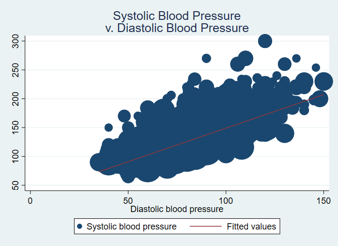
Analysis of subpopulations
Before we continue with our descriptive statistics, we should pause to discuss the analysis of subpopulations. The analysis of subpopulations is one place where survey data and experimental data are quite different. If you have data from an experiment (or quasi-experiment), and you want to analyze the responses from, say, just the women, or just people over age 50, you can just delete the unwanted cases from the data set or use the by: prefix. Complex survey data are different. With survey data, you (almost) never get to delete any cases from the data set, even if you will never use them in any of your analyses. Because of the way the -by- prefix works, you usually don’t use it with survey data either. (For an excellent discussion of conditional versus unconditional subdomain, please this presentation by Brady West, Ph.D.) Instead, Stata has provided two options that allow you to correctly analyze subpopulations of your survey data. These options are subpop and over. The subpop option is sort of like deleting unwanted cases (without really deleting them, of course), and the over option is very similar to -by- processing in that the output contains the estimates for each group. We will start with some examples of the subpop option. First, however, let’s take a second to see why deleting cases from a survey data set can be so problematic. If the data set is subset (meaning that observations not to be included in the subpopulation are deleted from the data set), the standard errors of the estimates cannot be calculated correctly. When the subpopulation option is used, only the cases defined by the subpopulation are used in the calculation of the estimate, but all cases are used in the calculation of the standard errors. For more information on this issue, please see Sampling Techniques, Third Edition by William G. Cochran (1977) and Small Area Estimation by J. N. K. Rao (2003). Also, if you look in the Stata 17 svy manual, you will find an entire section (pages 67-72) dedicated to the analysis of subpopulations. The formulas for using both if and subpop are given, along with an explanation of how they are different. If you look at the help for any svy: command, you will see the same warning:
Warning:  Use of if or in restrictions will not produce correct variance
      estimates for subpopulations in many cases.  To compute estimates for
      subpopulations, use the subpop() option.  The full specification for subpop()
      is
            subpop([varname] [if])
The subpop option on the svy: prefix without the if is used with binary
variables. (Technically, all cases coded as not 0 and not missing are part
of the subpopulation; this means that if your subpopulation variable has values
of 1 and 2, all of the observations will be included in the subpopulation unless
you use a different syntax.) You may need to create a binary variable
(using the generate command) in which all of the observations be to
included in the subpopulation are coded as 1 and all other observations are
coded as 0. For our example, we will use the variable female for
our subpopulation variable, so that only females will be included in calculation
of the point estimate.
svy: mean age
(running mean on estimation sample)

Survey: Mean estimation

Number of strata = 31            Number of obs   =      10,337
Number of PSUs   = 62            Population size = 117,023,659
                                 Design df       =          31

--------------------------------------------------------------
             |             Linearized
             |       Mean   std. err.     [95% conf. interval]
-------------+------------------------------------------------
         age |   42.23732   .3034412      41.61844    42.85619
--------------------------------------------------------------

svy, subpop(female): mean age
(running mean on estimation sample)

Survey: Mean estimation

Number of strata = 31            Number of obs   =      10,337
Number of PSUs   = 62            Population size = 117,023,659
                                 Subpop. no. obs =       5,428
                                 Subpop. size    =  60,901,624
                                 Design df       =          31

--------------------------------------------------------------
             |             Linearized
             |       Mean   std. err.     [95% conf. interval]
-------------+------------------------------------------------
         age |    42.5498   .3717231      41.79166    43.30793
--------------------------------------------------------------
To get the mean for the males, we can specify the subpopulation as the
variable female not equal to 1 (meaning the observations that are coded
0).
svy, subpop(if female != 1): mean age
(running mean on estimation sample)

Survey: Mean estimation

Number of strata = 31            Number of obs   =      10,337
Number of PSUs   = 62            Population size = 117,023,659
                                 Subpop. no. obs =       4,909
                                 Subpop. size    =  56,122,035
                                 Design df       =          31

--------------------------------------------------------------
             |             Linearized
             |       Mean   std. err.     [95% conf. interval]
-------------+------------------------------------------------
         age |   41.89822    .339303      41.20621    42.59024
--------------------------------------------------------------
We can also use the over option, which will give the results for each
level of the categorical variable listed. The over option is available only for svy: mean, svy: proportion,
svy: ratio and svy: total.
svy, over(female): mean age
(running mean on estimation sample)

Survey: Mean estimation

Number of strata = 31            Number of obs   =      10,337
Number of PSUs   = 62            Population size = 117,023,659
                                 Design df       =          31

--------------------------------------------------------------
             |             Linearized
             |       Mean   std. err.     [95% conf. interval]
-------------+------------------------------------------------
c.age@female |
       Male  |   41.89822    .339303      41.20621    42.59024
     Female  |    42.5498   .3717231      41.79166    43.30793
--------------------------------------------------------------
We can include more than one variable with the over option; this will
give us results for every combination of the variables listed.
svy, over(health female): mean copper
(running mean on estimation sample)

Survey: Mean estimation

Number of strata = 31                      Number of obs   =       9,116
Number of PSUs   = 62                      Population size = 103,479,298
                                           Design df       =          31

------------------------------------------------------------------------
                       |             Linearized
                       |       Mean   std. err.     [95% conf. interval]
-----------------------+------------------------------------------------
c.copper@health#female |
            Poor#Male  |   125.1899   1.800517      121.5177    128.8621
          Poor#Female  |   140.3425   2.196568      135.8626    144.8224
            Fair#Male  |   118.1246   1.288914      115.4958    120.7534
          Fair#Female  |   137.6154   1.273191      135.0187    140.2121
         Average#Male  |   113.7033   .9745251      111.7158    115.6909
       Average#Female  |   140.9529   1.780904      137.3207    144.5851
            Good#Male  |   108.7135   .6959349      107.2941    110.1328
          Good#Female  |   137.5177   1.374578      134.7142    140.3211
       Excellent#Male  |   106.3076   .5571644      105.1712    107.4439
     Excellent#Female  |   132.7433   1.569208      129.5429    135.9438
------------------------------------------------------------------------
We can also use the subpop option and the over option together.
In the example below, we get the mean of copper for females in each
combination of race and region (12 levels).
svy, subpop(female): mean copper, over(race region)
(running mean on estimation sample)

Survey: Mean estimation

Number of strata = 31                    Number of obs   =       9,677
Number of PSUs   = 62                    Population size = 109,683,584
                                         Subpop. no. obs =       4,768
                                         Subpop. size    =  53,561,549
                                         Design df       =          31

----------------------------------------------------------------------
                     |             Linearized
                     |       Mean   std. err.     [95% conf. interval]
---------------------+------------------------------------------------
c.copper@race#region |
           White#NE  |   133.8487   2.644552      128.4551    139.2423
           White#MW  |   135.3951   1.914987      131.4895    139.3008
            White#S  |   135.4202   1.677846      131.9982    138.8422
            White#W  |   140.4265   2.395216      135.5414    145.3115
           Black#NE  |   149.2318   3.040079      143.0315    155.4321
           Black#MW  |   146.0234   3.755621      138.3638     153.683
            Black#S  |   156.3648   4.922914      146.3245    166.4052
            Black#W  |   145.7466   1.902169      141.8671    149.6261
           Other#NE  |   103.1149   5.877161      91.12837    115.1015
           Other#MW  |   123.9078   5.761588      112.1569    135.6586
            Other#S  |   136.9562   19.24526      97.70521    176.2071
            Other#W  |   120.8002   1.899352      116.9265     124.674
----------------------------------------------------------------------
In some situations, no standard error or confidence intervals will be given.
This may be because there are very few observations at that level. To see if
this is indeed the cause, we can use the estat size command. The
unweighted number of cases is given in the column titled “Obs”, and the weighted
(or estimated subpopulation size) is given in the column titled “Size”.
estat size

----------------------------------------------------------------------
             |             Linearized
        Over |       Mean   std. err.              Obs            Size
-------------+--------------------------------------------------------
    c.copper@|
 race#region |
   White#NE  |   133.8487   2.644552               952      10,987,657
   White#MW  |   135.3951   1.914987             1,142      11,954,684
    White#S  |   135.4202   1.677846             1,099      12,006,761
    White#W  |   140.4265   2.395216             1,025      12,587,312
   Black#NE  |   149.2318   3.040079                52         576,302
   Black#MW  |   146.0234   3.755621               120       1,059,794
    Black#S  |   156.3648   4.922914               239       2,572,543
    Black#W  |   145.7466   1.902169                51         540,474
   Other#NE  |   103.1149   5.877161                 6          89,269
   Other#MW  |   123.9078   5.761588                 8         101,797
    Other#S  |   136.9562   19.24526                11         100,557
    Other#W  |   120.8002   1.899352                63         984,399
----------------------------------------------------------------------
The list command can be used to investigate combinations of subpopulation variables where the N is small.
The lincom command can be used to make comparisons between
subpopulations. In the first example below, we will compare the means for
males and females for iron. We
can use the display command to see how the point estimate in the output
of the lincom command is calculated. The value of using the
lincom command is that the standard error of point estimate is also
calculated, as well as the test statistic, p-value and 95% confidence interval. In
the following examples, we will compare the iron level
between males and females. Please see page 121 of the Stata
17 svy manual (first example in the section on survey post estimation) for more
information on using lincom after the svy, subpop(): mean command.
svy, over(female): mean iron
(running mean on estimation sample)

Survey: Mean estimation

Number of strata = 31             Number of obs   =      10,337
Number of PSUs   = 62             Population size = 117,023,659
                                  Design df       =          31

---------------------------------------------------------------
              |             Linearized
              |       Mean   std. err.     [95% conf. interval]
--------------+------------------------------------------------
c.iron@female |
        Male  |   104.8145   .5595657      103.6733    105.9558
      Female  |   97.17922   .6698075      95.81314     98.5453
---------------------------------------------------------------
We will need to add the coeflegend option to get Stata’s labels for the values we need.
svy, over(female): mean iron, coeflegend
(running mean on estimation sample)

Survey: Mean estimation

Number of strata = 31            Number of obs   =      10,337
Number of PSUs   = 62            Population size = 117,023,659
                                 Design df       =          31

-------------------------------------------------------------------------------
              |       Mean   Legend
--------------+----------------------------------------------------------------
c.iron@female |
        Male  |   104.8145  _b[c.iron@0bn.female]
      Female  |   97.17922  _b[c.iron@1.female]
-------------------------------------------------------------------------------

lincom _b[c.iron@0bn.female] - _b[c.iron@01.female]

 ( 1)  c.iron@0bn.female - c.iron@1.female = 0

------------------------------------------------------------------------------
        Mean | Coefficient  Std. err.      t    P>|t|     [95% conf. interval]
-------------+----------------------------------------------------------------
         (1) |   7.635327   .7467989    10.22   0.000     6.112221    9.158434
------------------------------------------------------------------------------
display 104.8145 - 97.17922 // a little rounding error 7.63528
In the next example, we compare different regions with respect to mean of copper.
svy, over(region): mean copper
(running mean on estimation sample)

Survey: Mean estimation

Number of strata = 31               Number of obs   =       9,118
Number of PSUs   = 62               Population size = 103,505,700
                                    Design df       =          31

-----------------------------------------------------------------
                |             Linearized
                |       Mean   std. err.     [95% conf. interval]
----------------+------------------------------------------------
c.copper@region |
            NE  |   122.5009     1.6006      119.2364    125.7653
            MW  |   123.5889   1.381478      120.7714    126.4064
             S  |   128.0201   1.162307      125.6495    130.3906
             W  |   124.3029   1.337444      121.5752    127.0306
-----------------------------------------------------------------

svy, over(region): mean copper, coeflegend
(running mean on estimation sample)

Survey: Mean estimation

Number of strata = 31            Number of obs   =       9,118
Number of PSUs   = 62            Population size = 103,505,700
                                 Design df       =          31

---------------------------------------------------------------------------------
                |       Mean   Legend
----------------+----------------------------------------------------------------
c.copper@region |
            NE  |   122.5009  _b[c.copper@1bn.region]
            MW  |   123.5889  _b[c.copper@2.region]
             S  |   128.0201  _b[c.copper@3.region]
             W  |   124.3029  _b[c.copper@4.region]
---------------------------------------------------------------------------------

lincom _b[c.copper@4.region] - _b[c.copper@1bn.region] // West - NE

 ( 1)  - c.copper@1bn.region + c.copper@4.region = 0

------------------------------------------------------------------------------
        Mean | Coefficient  Std. err.      t    P>|t|     [95% conf. interval]
-------------+----------------------------------------------------------------
         (1) |   1.802041   2.085828     0.86   0.394    -2.452033    6.056115
------------------------------------------------------------------------------

lincom _b[c.copper@4.region] - _b[c.copper@2.region] // West - MW

 ( 1)  - c.copper@2.region + c.copper@4.region = 0

------------------------------------------------------------------------------
        Mean | Coefficient  Std. err.      t    P>|t|     [95% conf. interval]
-------------+----------------------------------------------------------------
         (1) |   .7140072   1.922821     0.37   0.713    -3.207612    4.635626
------------------------------------------------------------------------------
We can use the svy: total command with either the subpop or the over option. The values in the output can get to be very large, so we can use the estimates table command to see them. We can also use the matrix list command.
svy, over(female): total diabetes
(running total on estimation sample)

Survey: Total estimation

Number of strata = 31                 Number of obs   =      10,335
Number of PSUs   = 62                 Population size = 116,997,257
                                      Design df       =          31

-------------------------------------------------------------------
                  |             Linearized
                  |      Total   std. err.     [95% conf. interval]
------------------+------------------------------------------------
c.diabetes@female |
            Male  |    1636958   159586.3       1311480     1962436
          Female  |    2374323   167874.1       2031941     2716705
-------------------------------------------------------------------

estimates table, b(%15.2f) se(%13.2f)

--------------------------------
    Variable |     Active
-------------+------------------
  c.diabetes@|
      female |
       Male  |      1636958.00
             |       159586.34
     Female  |      2374323.00
             |       167874.15
--------------------------------
                    Legend: b/se
Descriptive statistics with categorical variables
Let’s get some descriptive statistics with categorical variables. We
can use the svy: tabulate and svy: proportion commands. We will
use the region variable, region, which has four levels.
When used with no options, the output from the svy: tab command will give
us the same information as the svy: proportion command.
svy: tab region
(running tabulate on estimation sample)

Number of strata = 31                            Number of obs   =      10,337
Number of PSUs   = 62                            Population size = 117,023,659
                                                 Design df       =          31

----------------------
   Region | proportion
----------+-----------
       NE |      .2063
       MW |      .2492
        S |      .2656
        W |      .2789
          |
    Total |          1
----------------------
Key: proportion = Cell proportion
Let’s use some options with the svy: tab command so that we can see
the estimated number of people in each category.
svy: tab region, count cellwidth(12) format(%12.2g)
(running tabulate on estimation sample)

(running tabulate on estimation sample)

Number of strata = 31                            Number of obs   =      10,337
Number of PSUs   = 62                            Population size = 117,023,659
                                                 Design df       =          31

------------------------
   Region |        count
----------+-------------
       NE |     24146107
       MW |     29157970
        S |     31080884
        W |     32638698
          |
    Total |    117023659
------------------------
Key:        count = Weighted count
There are many options that can by used with svy: tab. Please
see the Stata help file for the svy: tabulate command for a complete
listing and description of each option. Only five items can be displayed
at once, and the ci option counts as two items.
svy: tab region, cell count obs cellwidth(12) format(%12.2g)
(running tabulate on estimation sample)

Number of strata = 31                            Number of obs   =      10,337
Number of PSUs   = 62                            Population size = 117,023,659
                                                 Design df       =          31

----------------------------------------------------
   Region |        count    proportion           obs
----------+-----------------------------------------
       NE |     24146107           .21          2086
       MW |     29157970           .25          2773
        S |     31080884           .27          2853
        W |     32638698           .28          2625
          |
    Total |    117023659             1         10337
----------------------------------------------------
Key:        count = Weighted count
       proportion = Cell proportion
              obs = Number of observations

svy: tab region, count se cellwidth(15) format(%15.2g)
(running tabulate on estimation sample)

Number of strata = 31                            Number of obs   =      10,337
Number of PSUs   = 62                            Population size = 117,023,659
                                                 Design df       =          31

--------------------------------------------
   Region |           count               se
----------+---------------------------------
       NE |        24146107           569293
       MW |        29157970           566351
        S |        31080884          1508325
        W |        32638698          1714567
          |
    Total |       117023659
--------------------------------------------
Key:           count = Weighted count
                  se = Linearized standard error of weighted count

svy: tab region, count deff deft ci cellwidth(12) format(%12.2g)
(running tabulate on estimation sample)

Number of strata = 31                            Number of obs   =      10,337
Number of PSUs   = 62                            Population size = 117,023,659
                                                 Design df       =          31

--------------------------------------------------------------------------------
   Region |        count            lb            ub          deff          deft
----------+---------------------------------------------------------------------
       NE |     24146107      22985026      25307188           1.5           1.2
       MW |     29157970      28002889      30313051           1.3           1.1
        S |     31080884      28004636      34157132           8.8             3
        W |     32638698      29141817      36135579            11           3.3
          |
    Total |    117023659
--------------------------------------------------------------------------------
Key:        count = Weighted count
               lb = Lower 95% confidence bound for weighted count
               ub = Upper 95% confidence bound for weighted count
             deff = DEFF for variance of weighted count
             deft = DEFT for variance of weighted count
Chi-square tests are provided by default when svy: tab is issued with
two variables. You will usually want to use the design-based test.
The proportion of observations in each cell can be obtained using either the
svy: tab or the svy: proportion command. If you want to compare
the proportions within two cells, you can use the lincom command.
svy: tab agegrp female, cell obs count cellwidth(12) format(%12.2g)
(running tabulate on estimation sample)

Number of strata = 31                            Number of obs   =      10,337
Number of PSUs   = 62                            Population size = 117,023,659
                                                 Design df       =          31

----------------------------------------------------
          |                  Female
Age group |         Male        Female         Total
----------+-----------------------------------------
    20–29 |     15918998      16938699      32857697
          |          .14           .14           .28
          |         1116          1204          2320
          |
    30–39 |     11777252      12150570      23927822
          |           .1            .1            .2
          |          770           851          1621
          |
    40–49 |      9538701      10152242      19690943
          |         .082          .087           .17
          |          610           660          1270
          |
    50–59 |      9210429      10337703      19548132
          |         .079          .088           .17
          |          601           688          1289
          |
    60–69 |      7326861       8261777      15588638
          |         .063          .071           .13
          |         1365          1487          2852
          |
      70+ |      2349794       3060633       5410427
          |          .02          .026          .046
          |          447           538           985
          |
    Total |     56122035      60901624     117023659
          |          .48           .52             1
          |         4909          5428         10337
----------------------------------------------------
Key: Weighted count
     Cell proportion
     Number of observations

  Pearson:
    Uncorrected   chi2(5)         =    6.7106
    Design-based  F(3.91, 121.15) =    1.2445     P = 0.2960

svy: proportion agegrp, over(female)
(running proportion on estimation sample)

Survey: Proportion estimation

Number of strata = 31             Number of obs   =      10,337
Number of PSUs   = 62             Population size = 117,023,659
                                  Design df       =          31

---------------------------------------------------------------
              |             Linearized            Logit
              | Proportion   std. err.     [95% conf. interval]
--------------+------------------------------------------------
agegrp@female |
  20–29 Male  |   .2836497   .0095365      .2646088    .3034953
20–29 Female  |   .2781321   .0085494      .2610357    .2958999
  30–39 Male  |   .2098508   .0086259      .1927991    .2279846
30–39 Female  |   .1995114   .0059814      .1875917    .2119909
  40–49 Male  |   .1699636   .0059311      .1582069    .1824046
40–49 Female  |    .166699   .0051213      .1565142    .1774073
  50–59 Male  |   .1641143   .0070436      .1502492    .1789894
50–59 Female  |   .1697443   .0068912      .1561486    .1842653
  60–69 Male  |   .1305523   .0051017       .120495    .1413141
60–69 Female  |   .1356577   .0040929      .1275246    .1442239
    70+ Male  |   .0418694   .0029631      .0362262    .0483475
  70+ Female  |   .0502554   .0038064      .0430362    .0586114
---------------------------------------------------------------

svy: proportion agegrp, over(female) coeflegend
(running proportion on estimation sample)

Survey: Proportion estimation

Number of strata = 31            Number of obs   =      10,337
Number of PSUs   = 62            Population size = 117,023,659
                                 Design df       =          31

-------------------------------------------------------------------------------
              | Proportion   Legend
--------------+----------------------------------------------------------------
agegrp@female |
  20–29 Male  |   .2836497  _b[1bn.agegrp@0bn.female]
20–29 Female  |   .2781321  _b[1bn.agegrp@1.female]
  30–39 Male  |   .2098508  _b[2.agegrp@0bn.female]
30–39 Female  |   .1995114  _b[2.agegrp@1.female]
  40–49 Male  |   .1699636  _b[3.agegrp@0bn.female]
40–49 Female  |    .166699  _b[3.agegrp@1.female]
  50–59 Male  |   .1641143  _b[4.agegrp@0bn.female]
50–59 Female  |   .1697443  _b[4.agegrp@1.female]
  60–69 Male  |   .1305523  _b[5.agegrp@0bn.female]
60–69 Female  |   .1356577  _b[5.agegrp@1.female]
    70+ Male  |   .0418694  _b[6.agegrp@0bn.female]
  70+ Female  |   .0502554  _b[6.agegrp@1.female]
-------------------------------------------------------------------------------

lincom _b[1bn.agegrp@0bn.female] - _b[1bn.agegrp@1.female] // (20-29 male) - (20-29 female)

( 1)  1bn.agegrp@0bn.female - 1bn.agegrp@1.female = 0

------------------------------------------------------------------------------
  Proportion | Coefficient  Std. err.      t    P>|t|     [95% conf. interval]
-------------+----------------------------------------------------------------
         (1) |   .0055176   .0108797     0.51   0.616    -.0166718    .0277069
------------------------------------------------------------------------------

display .2836497 - .2781321
.0055176
Graphs with categorical variables
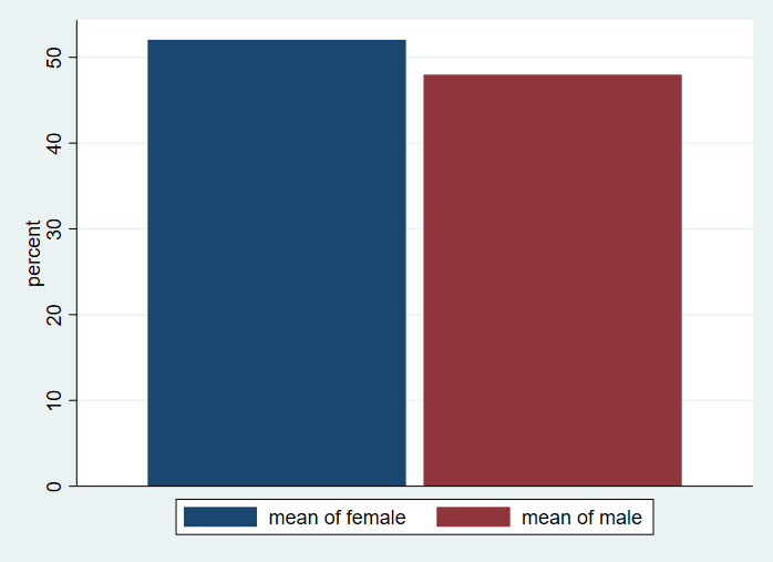
Let’s create a bar graph of the variable female. This graph will
show the percent of observations that are female and male. To do this, we
will need to create a new variable, which we will call male; it will
be the opposite of female.
gen male = !female
graph bar (mean) female male [pw = finalwgt], percentages bargap(7)
OLS regression
Now that we have descriptive statistics on our variables, we may want to run
some inferential statistics, such as OLS regression or logistic regression.
As before, we simply need to use the -svy- prefix before our regression commands.
Please note that the following analyses are shown only as examples of how to
do these analyses in Stata. There was no attempt to create substantively
meaningful models. Rather, the variables were chosen for illustrative
purposes only. We do not recommend that researchers create their models
this way.
We will start with an OLS regression with one categorical predictor (female). This is equivalent to a t-test. We will use the margins command get the means for each group. The vce(unconditional) option is used on all of the margins commands. This is the entry for this option from the Stata documentation:
vce(unconditional) specifies that the covariates that are not fixed be treated in a way that accounts for their having been sampled. The VCE is estimated using the linearization method. This method allows for heteroskedasticity or other violations of distributional assumptions and allows for correlation among the observations in the same manner as vce(robust) and vce(cluster…), which may have been specified with the estimation command. This method also accounts for complex survey designs if the data are svyset. See Obtaining margins with survey data and representative samples. When you use complex survey data, this method requires that the linearized variance estimation method be used for the model. See [SVY]svypostestimation for an example of margins with replication-based methods.
The coeflegend option is also used; this is a handy option that can be used with many Stata estimation commands and gives the labels that Stata assigns to these values. You use these labels to refer to the values when using commands such as lincom.
NOTE: If a regression is run on a subpopulation, the subpopulation must be specified as an option on the margins command if the desired output from margins is to the subpopulation.
Question: What do you call a linear regression with a single binary predictor?
Answer: A t-test!
There is no survey command for a t-test, but there are ways to do the equivalent of a t-test with survey data in Stata. Using the svy: regress command is equivalent to running a t-test assuming equal variances. Using either the svy: mean command with the over option, or using lincom produces a t-test assuming unequal variances.
svy: regress copper i.female
(running regress on estimation sample)

Survey: Linear regression

Number of strata = 31                            Number of obs   =       9,118
Number of PSUs   = 62                            Population size = 103,505,700
                                                 Design df       =          31
                                                 F(1, 31)        =      613.75
                                                 Prob > F        =      0.0000
                                                 R-squared       =      0.1489

------------------------------------------------------------------------------
             |             Linearized
      copper | Coefficient  std. err.      t    P>|t|     [95% conf. interval]
-------------+----------------------------------------------------------------
      female |
     Female  |   26.26294   1.060099    24.77   0.000     24.10085    28.42502
       _cons |   111.1328   .5685644   195.46   0.000     109.9732    112.2924
------------------------------------------------------------------------------

margins female, vce(unconditional)

Adjusted predictions

Number of strata = 31                            Number of obs   =       9,118
Number of PSUs   = 62                            Population size = 103,505,700
                                                 Design df       =          31

Expression: Linear prediction, predict()

------------------------------------------------------------------------------
             |             Linearized
             |     Margin   std. err.      t    P>|t|     [95% conf. interval]
-------------+----------------------------------------------------------------
      female |
       Male  |   111.1328   .5685644   195.46   0.000     109.9732    112.2924
     Female  |   137.3958   1.051281   130.69   0.000     135.2517    139.5399
------------------------------------------------------------------------------

display 137.3958 - 111.1328
26.263

margins female, vce(unconditional) coeflegend post // the post option is necessary when using the coeflegend option

Adjusted predictions

Number of strata = 31                            Number of obs   =       9,118
Number of PSUs   = 62                            Population size = 103,505,700
                                                 Design df       =          31

Expression: Linear prediction, predict()

------------------------------------------------------------------------------
             |     Margin   Legend
-------------+----------------------------------------------------------------
      female |
       Male  |   111.1328  _b[0bn.female]
     Female  |   137.3958  _b[1.female]
------------------------------------------------------------------------------

lincom _b[1.female] - _b[0bn.female]

 ( 1)  - 0bn.female + 1.female = 0

------------------------------------------------------------------------------
             | Coefficient  Std. err.      t    P>|t|     [95% conf. interval]
-------------+----------------------------------------------------------------
         (1) |   26.26294   1.060099    24.77   0.000     24.10085    28.42502
------------------------------------------------------------------------------
We can run the same t-test assuming unequal variances using the svy: mean and lincom commands.
svy, over(female): mean copper
(running mean on estimation sample)

Survey: Mean estimation

Number of strata = 31               Number of obs   =       9,118
Number of PSUs   = 62               Population size = 103,505,700
                                    Design df       =          31

-----------------------------------------------------------------
                |             Linearized
                |       Mean   std. err.     [95% conf. interval]
----------------+------------------------------------------------
c.copper@female |
          Male  |   111.1328   .5685644      109.9732    112.2924
        Female  |   137.3958   1.051281      135.2517    139.5399
-----------------------------------------------------------------

svy, over(female): mean copper, coeflegend
(running mean on estimation sample)

Survey: Mean estimation

Number of strata = 31            Number of obs   =       9,118
Number of PSUs   = 62            Population size = 103,505,700
                                 Design df       =          31

---------------------------------------------------------------------------------
                |       Mean   Legend
----------------+----------------------------------------------------------------
c.copper@female |
          Male  |   111.1328  _b[c.copper@0bn.female]
        Female  |   137.3958  _b[c.copper@1.female]
---------------------------------------------------------------------------------

lincom _b[c.copper@1.female] - _b[c.copper@0bn.female]

 ( 1)  - c.copper@0bn.female + c.copper@1.female = 0

------------------------------------------------------------------------------
        Mean | Coefficient  Std. err.      t    P>|t|     [95% conf. interval]
-------------+----------------------------------------------------------------
         (1) |   26.26294   1.060099    24.77   0.000     24.10085    28.42502
------------------------------------------------------------------------------
Let’s return to running linear regression models. We will add a continuous predictor to our OLS regression, so now the model has one categorical predictor (female) and one continuous predictor (age). In the output we see both the number of observations used in and the estimate of the size of the population. We see the overall test of the model and the R-squared for the model. The R-squared is the population R-squared and can be thought of as the adjusted R-squared. We will follow the svy: regress command with the margins command, which gives us the predicted values for each level of female.
svy: regress copper i.female age
(running regress on estimation sample)

Survey: Linear regression

Number of strata = 31                            Number of obs   =       9,118
Number of PSUs   = 62                            Population size = 103,505,700
                                                 Design df       =          31
                                                 F(2, 30)        =      448.23
                                                 Prob > F        =      0.0000
                                                 R-squared       =      0.1497

------------------------------------------------------------------------------
             |             Linearized
      copper | Coefficient  std. err.      t    P>|t|     [95% conf. interval]
-------------+----------------------------------------------------------------
      female |
     Female  |   26.20177   1.087402    24.10   0.000       23.984    28.41954
         age |   .0635486   .0330805     1.92   0.064    -.0039196    .1310168
       _cons |   108.4748   1.540579    70.41   0.000     105.3327    111.6168
------------------------------------------------------------------------------

margins female, vce(unconditional)

Predictive margins

Number of strata = 31                            Number of obs   =       9,118
Number of PSUs   = 62                            Population size = 103,505,700
                                                 Design df       =          31

Expression: Linear prediction, predict()

------------------------------------------------------------------------------
             |             Linearized
             |     Margin   std. err.      t    P>|t|     [95% conf. interval]
-------------+----------------------------------------------------------------
      female |
       Male  |   111.1645   .5718949   194.38   0.000     109.9981    112.3309
     Female  |   137.3663   1.062916   129.24   0.000     135.1984    139.5341
------------------------------------------------------------------------------
Now let’s run a model with a categorical by categorical (specifically a binary by binary) interaction term.
We can use the contrast command to get the test of the interaction
displayed as an F-test rather than a t-statistic. Of course, the p-value
is exactly the same as the one shown in the table of coefficients because the test of a binary by binary interaction is a one degree-of-freedom test. We can use the margins command to get the predicted
values of copper for each combination of female and diabetes.
The marginsplot
command is used to obtain a graph of the interaction (marginsplot graphs the values shown
in the output from the margins command).
svy: regress copper i.female##i.diabetes age
(running regress on estimation sample)

Survey: Linear regression

Number of strata = 31                            Number of obs   =       9,116
Number of PSUs   = 62                            Population size = 103,479,298
                                                 Design df       =          31
                                                 F(4, 28)        =      315.94
                                                 Prob > F        =      0.0000
                                                 R-squared       =      0.1505

----------------------------------------------------------------------------------
                 |             Linearized
          copper | Coefficient  std. err.      t    P>|t|     [95% conf. interval]
-----------------+----------------------------------------------------------------
          female |
         Female  |   26.42748   1.091601    24.21   0.000     24.20114    28.65381
                 |
        diabetes |
       Diabetic  |   6.350642   2.034884     3.12   0.004     2.200469    10.50082
                 |
 female#diabetes |
Female#Diabetic  |  -6.493926   2.706082    -2.40   0.023    -12.01302   -.9748357
                 |
             age |   .0573067   .0332424     1.72   0.095    -.0104917    .1251051
           _cons |   108.5489   1.542311    70.38   0.000     105.4034    111.6945
----------------------------------------------------------------------------------

contrast female#diabetes, effects

Contrasts of marginal linear predictions

                                                                Design df = 31

Margins: asbalanced

---------------------------------------------------
                |         df           F        P>F
----------------+----------------------------------
female#diabetes |          1        5.76     0.0226
         Design |         31
---------------------------------------------------
Note: F statistics are adjusted for the survey
      design.

------------------------------------------------------------------------------------------------------
                                     |   Contrast   Std. err.      t    P>|t|     [95% conf. interval]
-------------------------------------+----------------------------------------------------------------
                     female#diabetes |
(Female vs base) (Diabetic vs base)  |  -6.493926   2.706082    -2.40   0.023    -12.01302   -.9748357
------------------------------------------------------------------------------------------------------

margins female#diabetes, vce(unconditional)

Predictive margins

Number of strata = 31                            Number of obs   =       9,116
Number of PSUs   = 62                            Population size = 103,479,298
                                                 Design df       =          31

Expression: Linear prediction, predict()

--------------------------------------------------------------------------------------
                     |             Linearized
                     |     Margin   std. err.      t    P>|t|     [95% conf. interval]
---------------------+----------------------------------------------------------------
     female#diabetes |
  Male#Not diabetic  |   110.9745   .5531673   200.62   0.000     109.8463    112.1027
      Male#Diabetic  |   117.3252   2.201312    53.30   0.000     112.8356    121.8148
Female#Not diabetic  |    137.402   1.077068   127.57   0.000     135.2053    139.5987
    Female#Diabetic  |   137.2587   2.417731    56.77   0.000     132.3277    142.1897
-------------------------------------------------------------------------------------
marginsplot Variables that uniquely identify margins: female diabetes
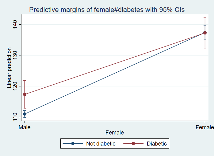
Some of you may recognize this analysis as a “difference-in-differences” analysis. In other words, the term of interest is the binary-by-binary interaction term. Let’s reproduce the coefficient of this interaction term, -6.493926, by taking the difference of the differences ((male_no – male_yes) -(female_no – female_yes)). First, we need to need to rerun the margins command with the coeflegend option and the post option; the post option is needed so that we can access the values remembered by margins with another command. The output will show us the names of the values. We will use these names rather than the actual values themselves, so that if the data or model were changed, the code would not need to be modified. We will use the lincom command to do the math for us. The advantage of using the lincom command over the display command is that lincom will also produce the standard error.
margins female#diabetes, vce(unconditional)

Predictive margins

Number of strata = 31                            Number of obs   =       9,116
Number of PSUs   = 62                            Population size = 103,479,298
                                                 Design df       =          31

Expression: Linear prediction, predict()

--------------------------------------------------------------------------------------
                     |             Linearized
                     |     Margin   std. err.      t    P>|t|     [95% conf. interval]
---------------------+----------------------------------------------------------------
     female#diabetes |
  Male#Not diabetic  |   110.9745   .5531673   200.62   0.000     109.8463    112.1027
      Male#Diabetic  |   117.3252   2.201312    53.30   0.000     112.8356    121.8148
Female#Not diabetic  |    137.402   1.077068   127.57   0.000     135.2053    139.5987
    Female#Diabetic  |   137.2587   2.417731    56.77   0.000     132.3277    142.1897
--------------------------------------------------------------------------------------
margins, vce(unconditional) coeflegend post Predictive margins Number of strata = 31 Number of obs = 9,116 Number of PSUs = 62 Population size = 103,479,298 Design df = 31 Expression: Linear prediction, predict() -------------------------------------------------------------------------------------- | Linearized | Margin std. err. t P>|t| [95% conf. interval] ---------------------+---------------------------------------------------------------- female#diabetes | Male#Not diabetic | 110.9745 .5531673 200.62 0.000 109.8463 112.1027 Male#Diabetic | 117.3252 2.201312 53.30 0.000 112.8356 121.8148 Female#Not diabetic | 137.402 1.077068 127.57 0.000 135.2053 139.5987 Female#Diabetic | 137.2587 2.417731 56.77 0.000 132.3277 142.1897 --------------------------------------------------------------------------------------lincom (_b[0bn.female#0bn.diabetes]-_b[0bn.female#1.diabetes]) - (_b[1.female#0bn.diabetes]-_b[1.female#1.diabetes]) ( 1) 0bn.female#0bn.diabetes - 0bn.female#1.diabetes - 1.female#0bn.diabetes + 1.female#1.diabetes = 0 ------------------------------------------------------------------------------ | Coefficient Std. err. t P>|t| [95% conf. interval] -------------+---------------------------------------------------------------- (1) | -6.493926 2.706082 -2.40 0.023 -12.01302 -.9748357 ------------------------------------------------------------------------------
We can see that the output from the lincom command is the same as the output for the interaction term in the original regression command.
Looking back at the graph of the interaction, you may wonder if the two points for male are statistically significantly different from one another, and the same for the two points for females. The lincom command can be used for these comparisons.
* males
lincom (_b[0bn.female#0bn.diabetes]-_b[0bn.female#1.diabetes])

 ( 1)  0bn.female#0bn.diabetes - 0bn.female#1.diabetes = 0

------------------------------------------------------------------------------
             | Coefficient  Std. err.      t    P>|t|     [95% conf. interval]
-------------+----------------------------------------------------------------
         (1) |  -6.350642   2.034884    -3.12   0.004    -10.50082   -2.200469
------------------------------------------------------------------------------

* females
lincom (_b[1.female#0bn.diabetes]-_b[1.female#1.diabetes])

 ( 1)  1.female#0bn.diabetes - 1.female#1.diabetes = 0

------------------------------------------------------------------------------
             | Coefficient  Std. err.      t    P>|t|     [95% conf. interval]
-------------+----------------------------------------------------------------
         (1) |   .1432847    2.42126     0.06   0.953    -4.794907    5.081476
------------------------------------------------------------------------------
In the next example, we will use a categorical by continuous interaction.
In the first call to the margins command, we get the simple slope
coefficients for males and females. The p-values in this table tell us
that both slopes are significantly different from 0. In the second call to the margins
command, we get the predicted values for each level of female at height =
140, height = 150, height = 160, up to height = 190. The t-statistics and
corresponding p-values tell us if the predicted value is different from 0.
svy: regress bpsystol i.female##c.height
(running regress on estimation sample)

Survey: Linear regression

Number of strata = 31                            Number of obs   =      10,337
Number of PSUs   = 62                            Population size = 117,023,659
                                                 Design df       =          31
                                                 F(3, 29)        =       71.21
                                                 Prob > F        =      0.0000
                                                 R-squared       =      0.0309

---------------------------------------------------------------------------------
                |             Linearized
       bpsystol | Coefficient  std. err.      t    P>|t|     [95% conf. interval]
----------------+----------------------------------------------------------------
         female |
        Female  |   43.61115   13.30799     3.28   0.003     16.46933    70.75298
         height |  -.1647344   .0518262    -3.18   0.003    -.2704347   -.0590342
                |
female#c.height |
        Female  |  -.3185637   .0785976    -4.05   0.000    -.4788646   -.1582627
                |
          _cons |   158.8447   9.148233    17.36   0.000     140.1868    177.5026
---------------------------------------------------------------------------------

margins female, dydx(height) vce(unconditional)

Average marginal effects

Number of strata = 31                            Number of obs   =      10,337
Number of PSUs   = 62                            Population size = 117,023,659
                                                 Design df       =          31

Expression: Linear prediction, predict()
dy/dx wrt:  height

------------------------------------------------------------------------------
             |             Linearized
             |      dy/dx   std. err.      t    P>|t|     [95% conf. interval]
-------------+----------------------------------------------------------------
height       |
      female |
       Male  |  -.1647344   .0518262    -3.18   0.003    -.2704347   -.0590342
     Female  |  -.4832981   .0550113    -8.79   0.000    -.5954944   -.3711018
------------------------------------------------------------------------------

margins female, at(height=(140(10)190)) vsquish vce(unconditional)

Adjusted predictions

Number of strata = 31                            Number of obs   =      10,337
Number of PSUs   = 62                            Population size = 117,023,659
                                                 Design df       =          31

Expression: Linear prediction, predict()
1._at: height = 140
2._at: height = 150
3._at: height = 160
4._at: height = 170
5._at: height = 180
6._at: height = 190

------------------------------------------------------------------------------
             |             Linearized
             |     Margin   std. err.      t    P>|t|     [95% conf. interval]
-------------+----------------------------------------------------------------
  _at#female |
     1#Male  |   135.7819   1.978535    68.63   0.000     131.7466    139.8171
   1#Female  |   134.7941   1.501944    89.75   0.000     131.7309    137.8574
     2#Male  |   134.1345   1.498425    89.52   0.000     131.0785    137.1906
   2#Female  |   129.9611   1.046223   124.22   0.000     127.8274    132.0949
     3#Male  |   132.4872   1.055057   125.57   0.000     130.3354     134.639
   3#Female  |   125.1282   .7338792   170.50   0.000     123.6314    126.6249
     4#Male  |   130.8399   .7198653   181.76   0.000     129.3717     132.308
   4#Female  |   120.2952   .7666958   156.90   0.000     118.7315    121.8589
     5#Male  |   129.1925   .6785699   190.39   0.000     127.8086    130.5765
   5#Female  |   115.4622   1.114592   103.59   0.000      113.189    117.7354
     6#Male  |   127.5452   .9694841   131.56   0.000     125.5679    129.5224
   6#Female  |   110.6292   1.581789    69.94   0.000     107.4031    113.8553
------------------------------------------------------------------------------
marginsplot
Variables that uniquely identify margins: height female
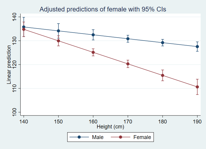
In the example below, we get the difference between the predicted values for
males and females at six values of height. We then use the
marginsplot command to graph these differences. This graph shows that
the difference between males and females is larger at the extreme values of
height, as is the variability around those estimates.
Notice that in the output from the margins command above, the
predicted value for 4#female is 120.2952 and the predicted value for 4#male
is 130.8399. 120.2952-130.8399 = -10.5447, which is the value of dy/dx
on line 4 of the output below.
margins, dydx(female) at(height=(140(10)190)) vsquish vce(unconditional)

Conditional marginal effects

Number of strata = 31                            Number of obs   =      10,337
Number of PSUs   = 62                            Population size = 117,023,659
                                                 Design df       =          31

Expression: Linear prediction, predict()
dy/dx wrt:  1.female
1._at: height = 140
2._at: height = 150
3._at: height = 160
4._at: height = 170
5._at: height = 180
6._at: height = 190

------------------------------------------------------------------------------
             |             Linearized
             |      dy/dx   std. err.      t    P>|t|     [95% conf. interval]
-------------+----------------------------------------------------------------
0.female     |  (base outcome)
-------------+----------------------------------------------------------------
1.female     |
         _at |
          1  |  -.9877624   2.392115    -0.41   0.683    -5.866514    3.890989
          2  |  -4.173399   1.657451    -2.52   0.017    -7.553793   -.7930051
          3  |  -7.359036   1.003788    -7.33   0.000    -9.406275   -5.311796
          4  |  -10.54467   .7096161   -14.86   0.000    -11.99194   -9.097401
          5  |  -13.73031   1.111322   -12.35   0.000    -15.99687   -11.46375
          6  |  -16.91595   1.789424    -9.45   0.000     -20.5655   -13.26639
------------------------------------------------------------------------------
Note: dy/dx for factor levels is the discrete change from the base level.
marginsplot, yline(0) Variables that uniquely identify margins: height
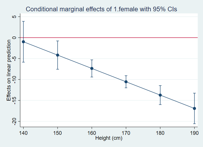
Let’s remake this graph with confidence interval as an area plot.
marginsplot, yline(0) recast(line) recastci(rarea) ciopts(color(*.2))

  Variables that uniquely identify margins: height
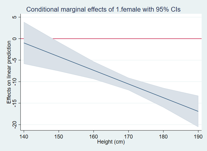
If we use a categorical predictor variable in our model that has more than
two levels, we may want to run comparisons between each of the levels. In
the example below, we use the region variable, region,
as a predictor. We use the contrast command to determine if, taken
together, region, is a statistically significant predictor of our
outcome variable, copper. Next, we use the pwcompare command
to conduct all pairwise comparisons. We use the mcompare(sidak)
option to adjust the p-values for the multiple comparisons, and we use the
pveffects option to have the test statistics and p-values shown in the
output. Other options that we could have used with the mcompare
option are bonferroni and scheffe.
svy: regress copper i.region age
(running regress on estimation sample)

Survey: Linear regression

Number of strata = 31                            Number of obs   =       9,118
Number of PSUs   = 62                            Population size = 103,505,700
                                                 Design df       =          31
                                                 F(4, 28)        =        3.93
                                                 Prob > F        =      0.0118
                                                 R-squared       =      0.0054

------------------------------------------------------------------------------
             |             Linearized
      copper | Coefficient  std. err.      t    P>|t|     [95% conf. interval]
-------------+----------------------------------------------------------------
      region |
         MW  |   1.222524   2.098883     0.58   0.564    -3.058175    5.503223
          S  |   5.527657    1.97134     2.80   0.009     1.507083    9.548231
          W  |   1.951666   2.093714     0.93   0.358    -2.318492    6.221824
             |
         age |   .0878814   .0359642     2.44   0.020     .0145319    .1612308
       _cons |    118.706   2.487797    47.72   0.000     113.6322    123.7799
------------------------------------------------------------------------------

contrast region

Contrasts of marginal linear predictions

                                                                Design df = 31

Margins: asbalanced

------------------------------------------------
             |         df           F        P>F
-------------+----------------------------------
      region |          3        3.23     0.0368
      Design |         31
------------------------------------------------
Note: F statistics are adjusted for the survey
      design.

pwcompare region, mcompare(sidak) cformat(%3.1f) pveffects

Pairwise comparisons of marginal linear predictions

                                                                Design df = 31

Margins: asbalanced

---------------------------
             |    Number of
             |  comparisons
-------------+-------------
      region |            6
---------------------------

-----------------------------------------------------
             |                              Sidak
             |   Contrast   Std. err.      t    P>|t|
-------------+---------------------------------------
      region |
   MW vs NE  |        1.2        2.1     0.58   0.993
    S vs NE  |        5.5        2.0     2.80   0.051
    W vs NE  |        2.0        2.1     0.93   0.930
    S vs MW  |        4.3        1.8     2.42   0.123
    W vs MW  |        0.7        1.9     0.38   0.999
     W vs S  |       -3.6        1.8    -2.02   0.277
-----------------------------------------------------
Let’s see what a regression looks like for a subpopulation.
svy, subpop(if region == 1): regress copper i.female age
(running regress on estimation sample)

Survey: Linear regression

Number of strata =  7                             Number of obs   =      1,962
Number of PSUs   = 14                             Population size = 22,845,478
                                                  Subpop. no. obs =      1,962
                                                  Subpop. size    = 22,845,478
                                                  Design df       =          7
                                                  F(2, 6)         =      89.39
                                                  Prob > F        =     0.0000
                                                  R-squared       =     0.1450

------------------------------------------------------------------------------
             |             Linearized
      copper | Coefficient  std. err.      t    P>|t|     [95% conf. interval]
-------------+----------------------------------------------------------------
      female |
     Female  |   24.21052    1.85708    13.04   0.000     19.81923    28.60182
         age |   .0658891   .0668075     0.99   0.357    -.0920855    .2238638
       _cons |   107.3062   3.550041    30.23   0.000     98.91166    115.7007
------------------------------------------------------------------------------
Note: 24 strata omitted because they contain no subpopulation members.

margins female, vce(unconditional) subpop(if region == 1)

Predictive margins

Number of strata =  7                             Number of obs   =      1,962
Number of PSUs   = 14                             Population size = 22,845,478
                                                  Subpop. no. obs =      1,962
                                                  Subpop. size    =          .
                                                  Design df       =          7

Expression: Linear prediction, predict()

------------------------------------------------------------------------------
             |             Linearized
             |     Margin   std. err.      t    P>|t|     [95% conf. interval]
-------------+----------------------------------------------------------------
      female |
       Male  |   110.1513   1.243823    88.56   0.000     107.2102    113.0925
     Female  |   134.3619   2.456248    54.70   0.000     128.5538      140.17
------------------------------------------------------------------------------
Logistic regression
Let’s run a logistic regression. We will use the variable highbp
(Do you have high blood pressure?)
as the outcome variable. Before we run our logistic regression, let’s look at
the distribution of the outcome variable, and let’s look at the crosstabulation
of the outcome variable with our categorical predictor variable. The
purpose of the first descriptive analysis is to assess the proportion and number
of cases in each level of the outcome variable. If we found that there was
a very small proportion of cases in one of the levels, we may encounter
estimation problems with the logistic regression. Likewise, if the
crosstabulation between the outcome variable and the categorical predictor
variable showed that one or more cells had very few unweighted observations or
no observations at all, we might want to recode the predictor variable into
fewer categories so that there were a sufficient number of observations in each
cell. The results below do not look problematic, although there are
relatively few observations that are coded as 0 on our outcome variable and 1 on
our predictor variable. This might increase the standard error around that
point estimate.
svy: tab highbp, cell obs count cellwidth(12) format(%12.2g)
(running tabulate on estimation sample)

Number of strata = 31                            Number of obs   =      10,337
Number of PSUs   = 62                            Population size = 117,023,659
                                                 Design df       =          31

----------------------------------------------------
High      |
blood     |
pressure  |        count    proportion           obs
----------+-----------------------------------------
        0 |     73871969           .63          5965
        1 |     43151690           .37          4372
          |
    Total |    117023659             1         10337
----------------------------------------------------
Key:        count = Weighted count
       proportion = Cell proportion
              obs = Number of observations

svy: tab health highbp, cell obs count cellwidth(12) format(%12.2g)
(running tabulate on estimation sample)

Number of strata = 31                            Number of obs   =      10,335
Number of PSUs   = 62                            Population size = 116,997,257
                                                 Design df       =          31

----------------------------------------------------
1=poor,.. |
.,        |
5=excelle |           High blood pressure
nt        |            0             1         Total
----------+-----------------------------------------
     Poor |      2550049       2987907       5537956
          |         .022          .026          .047
          |          310           419           729
          |
     Fair |      7370803       7009458      14380261
          |         .063           .06           .12
          |          766           904          1670
          |
  Average |     19137093      13578302      32715395
          |          .16           .12           .28
          |         1572          1366          2938
          |
     Good |     21856626      10319684      32176310
          |          .19          .088           .28
          |         1666           925          2591
          |
 Excellen |     22930996       9256339      32187335
          |           .2          .079           .28
          |         1649           758          2407
          |
    Total |     73845567      43151690     116997257
          |          .63           .37             1
          |         5963          4372         10335
----------------------------------------------------
Key: Weighted count
     Cell proportion
     Number of observations

  Pearson:
    Uncorrected   chi2(4)         =  273.4001
    Design-based  F(3.53, 109.46) =   49.8959     P = 0.0000
Now let’s run the logistic regression. We can use the contrast command
to get the multi-degree-of-freedom test of health (which is statistically significant). Note that the logistic regression coefficients are interpreted the same way that they are in an unweighted model.
svy: logit highbp ib3.health c.age
(running logit on estimation sample)

Survey: Logistic regression

Number of strata = 31                            Number of obs   =      10,335
Number of PSUs   = 62                            Population size = 116,997,257
                                                 Design df       =          31
                                                 F(5, 27)        =      186.86
                                                 Prob > F        =      0.0000

------------------------------------------------------------------------------
             |             Linearized
      highbp | Coefficient  std. err.      t    P>|t|     [95% conf. interval]
-------------+----------------------------------------------------------------
      health |
       Poor  |   .0422165   .1317361     0.32   0.751    -.2264609     .310894
       Fair  |   .0015363   .0676718     0.02   0.982    -.1364811    .1395538
       Good  |  -.1926015   .0614354    -3.14   0.004    -.3178998   -.0673033
  Excellent  |  -.2633746   .0769005    -3.42   0.002    -.4202142    -.106535
             |
         age |   .0473091   .0015249    31.03   0.000     .0441992    .0504191
       _cons |  -2.480283   .1060894   -23.38   0.000    -2.696654   -2.263913
------------------------------------------------------------------------------

contrast health

Contrasts of marginal linear predictions

                                                                Design df = 31

Margins: asbalanced

------------------------------------------------
             |         df           F        P>F
-------------+----------------------------------
      health |          4        3.85     0.0129
      Design |         31
------------------------------------------------
Note: F statistics are adjusted for the survey
      design.
Let’s include a categorical by continuous interaction in the model. We
will use the contrast command to determine if the interaction term (as a
whole) is statistically significant. We will use the contrast
command to get the multi-degree-of-freedom test of the interaction, the margins
command to get the predicted probabilities and the marginsplot command
to graph the interaction.
svy: logit highbp ib3.health##c.age
(running logit on estimation sample)

Survey: Logistic regression

Number of strata = 31                            Number of obs   =      10,335
Number of PSUs   = 62                            Population size = 116,997,257
                                                 Design df       =          31
                                                 F(9, 23)        =       86.76
                                                 Prob > F        =      0.0000

------------------------------------------------------------------------------
             |             Linearized
      highbp | Coefficient  std. err.      t    P>|t|     [95% conf. interval]
-------------+----------------------------------------------------------------
      health |
       Poor  |   1.184622   .4603688     2.57   0.015     .2456932     2.12355
       Fair  |   .0943241   .2754073     0.34   0.734    -.4673728     .656021
       Good  |  -.3275786   .1702732    -1.92   0.064    -.6748529    .0196958
  Excellent  |  -.4030749   .1921477    -2.10   0.044    -.7949627    -.011187
             |
         age |   .0467356   .0025779    18.13   0.000     .0414779    .0519933
             |
health#c.age |
       Poor  |  -.0206937   .0078239    -2.64   0.013    -.0366506   -.0047367
       Fair  |  -.0017234   .0052911    -0.33   0.747    -.0125146    .0090678
       Good  |   .0031633   .0035254     0.90   0.376    -.0040267    .0103534
  Excellent  |   .0033972   .0040242     0.84   0.405    -.0048104    .0116047
             |
       _cons |  -2.453943   .1458084   -16.83   0.000    -2.751322   -2.156565
------------------------------------------------------------------------------

contrast health#c.age

Contrasts of marginal linear predictions

                                                                Design df = 31

Margins: asbalanced

------------------------------------------------
             |         df           F        P>F
-------------+----------------------------------
health#c.age |          4        2.54     0.0617
      Design |         31
------------------------------------------------
Note: F statistics are adjusted for the survey
      design.

contrast health

Contrasts of marginal linear predictions

                                                                Design df = 31

Margins: asbalanced

------------------------------------------------
             |         df           F        P>F
-------------+----------------------------------
      health |          4        3.58     0.0176
      Design |         31
------------------------------------------------
Note: F statistics are adjusted for the survey
      design.
margins health, at(age=(20(10)70)) vsquish vce(unconditional) Adjusted predictions Number of strata = 31 Number of obs = 10,335 Number of PSUs = 62 Population size = 116,997,257 Design df = 31 Expression: Pr(highbp), predict() 1._at: age = 20 2._at: age = 30 3._at: age = 40 4._at: age = 50 5._at: age = 60 6._at: age = 70 ------------------------------------------------------------------------------ | Linearized | Margin std. err. t P>|t| [95% conf. interval] -------------+---------------------------------------------------------------- _at#health | 1#Poor | .321152 .0676631 4.75 0.000 .1831522 .4591517 1#Fair | .188563 .0273867 6.89 0.000 .1327074 .2444185 1#Average | .1795748 .0154403 11.63 0.000 .1480841 .2110655 1#Good | .1438662 .0112541 12.78 0.000 .1209134 .1668191 1#Excellent | .1353615 .0128287 10.55 0.000 .1091971 .1615258 2#Poor | .3803499 .0579559 6.56 0.000 .2621481 .4985517 2#Fair | .2671262 .0280849 9.51 0.000 .2098467 .3244057 2#Average | .2588653 .0169863 15.24 0.000 .2242214 .2935091 2#Good | .2167762 .0129495 16.74 0.000 .1903655 .2431868 2#Excellent | .2053746 .0157743 13.02 0.000 .1732028 .2375465 3#Poor | .4433335 .0459814 9.64 0.000 .3495538 .5371132 3#Fair | .3637487 .0263469 13.81 0.000 .3100139 .4174836 3#Average | .3578936 .0178355 20.07 0.000 .3215178 .3942693 3#Good | .313122 .0151767 20.63 0.000 .2821689 .3440752 3#Excellent | .2990749 .0197526 15.14 0.000 .2587891 .3393607 4#Poor | .5081932 .0345058 14.73 0.000 .4378182 .5785682 4#Fair | .472775 .0238764 19.80 0.000 .4240788 .5214711 4#Average | .4707429 .0185394 25.39 0.000 .4329315 .5085543 4#Good | .4288428 .0187103 22.92 0.000 .3906828 .4670028 4#Excellent | .4132904 .0249908 16.54 0.000 .3623213 .4642596 5#Poor | .5727782 .0284395 20.14 0.000 .5147755 .6307808 5#Fair | .5844612 .0233301 25.05 0.000 .5368791 .6320432 5#Average | .5866646 .0193689 30.29 0.000 .5471616 .6261677 5#Good | .5529051 .0226358 24.43 0.000 .5067391 .5990711 5#Excellent | .5376656 .0300081 17.92 0.000 .4764636 .5988677 6#Poor | .6349738 .0311436 20.39 0.000 .571456 .6984917 6#Fair | .6880968 .0245797 27.99 0.000 .6379662 .7382274 6#Average | .6937161 .019649 35.31 0.000 .6536417 .7337905 6#Good | .6707116 .0248188 27.02 0.000 .6200934 .7213298 6#Excellent | .6575232 .032423 20.28 0.000 .5913962 .7236503 ------------------------------------------------------------------------------ marginsplot Variables that uniquely identify margins: age health
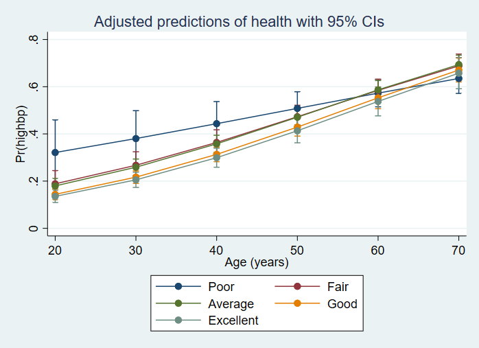
Next, we will run a logistic regression model and use the
estat gof command to get the Archer-Lemeshow test (which is a modification
of the Hosmer-Lemeshow test that can be used with survey data). The
numerator degrees of freedom are calculated as g – 1, and the denominator
degrees of freedom are calculated as f – g + 2, where f = the number of sampled
clusters – the number of strata and g = the number of groups (10 is the
default). For the following example, we have 10 – 1 = 9 numerator degrees
of freedom and 31 – 10 + 2 = 23 denominator degrees of freedom. In the output below,
we see that the Archer-Lemeshow test is not statistically significant. This suggests
that the model fit is acceptable. As of Stata 17, estat gof cannot follow a model specified with a
subpopulation.
svy: logit highbp i.female##c.age
(running logit on estimation sample)

Number of strata = 31                            Number of obs   =      10,337
Number of PSUs   = 62                            Population size = 117,023,659
                                                 Design df       =          31
                                                 F(3, 29)        =      335.03
                                                 Prob > F        =      0.0000

------------------------------------------------------------------------------
             |             Linearized
      highbp | Coefficient  std. err.      t    P>|t|     [95% conf. interval]
-------------+----------------------------------------------------------------
      female |
     Female  |  -1.922498   .1940278    -9.91   0.000    -2.318221   -1.526776
         age |     .03707   .0023869    15.53   0.000     .0322019    .0419381
             |
female#c.age |
     Female  |   .0294389   .0040073     7.35   0.000      .021266    .0376118
             |
       _cons |  -1.863043   .1414675   -13.17   0.000    -2.151567   -1.574518
------------------------------------------------------------------------------

estat gof

Logistic model for highbp, goodness-of-fit test

                      F(9,23) =         2.06
                     Prob > F =         0.0784
Ordinal Logistic Regression
Here is an example of an ordinal logistic regression. The outcome variable, health, has ordered categories, but it is not a continuous variable. In the first call, we get the coefficients in the log-odds metric. In the second call, we request odds ratios. The discussion of ordinal logistic regression will be minimal; for more information regarding ordinal logistic regression, please see our Stata Data Analysis Examples: Ordinal Logistic Regression and Stata Annotated Output: Ordinal Logistic Regression. Although these pages show examples that use non-weighted data, they are still helpful because the interpretation of the coefficients is the same with weighted and non-weighted data.
svy: ologit health i.female i.region age
(running ologit on estimation sample)

Survey: Ordered logistic regression

Number of strata = 31                            Number of obs   =      10,335
Number of PSUs   = 62                            Population size = 116,997,257
                                                 Design df       =          31
                                                 F(5, 27)        =      135.54
                                                 Prob > F        =      0.0000

------------------------------------------------------------------------------
             |             Linearized
      health | Coefficient  std. err.      t    P>|t|     [95% conf. interval]
-------------+----------------------------------------------------------------
      female |
     Female  |  -.1696374   .0493449    -3.44   0.002    -.2702769   -.0689979
             |
      region |
         MW  |   -.115146   .1030587    -1.12   0.272    -.3253356    .0950437
          S  |  -.5365581   .1050491    -5.11   0.000    -.7508071   -.3223091
          W  |  -.2887877   .1019162    -2.83   0.008    -.4966471   -.0809283
             |
         age |  -.0397158   .0014944   -26.58   0.000    -.0427636   -.0366681
-------------+----------------------------------------------------------------
       /cut1 |  -5.210696    .122255                     -5.460036   -4.961355
       /cut2 |  -3.717526   .1126799                     -3.947339   -3.487714
       /cut3 |  -2.202685   .1097316                     -2.426484   -1.978886
       /cut4 |  -.9350942   .1089012                       -1.1572   -.7129888
------------------------------------------------------------------------------

contrast region

Contrasts of marginal linear predictions

                                                                Design df = 31

Margins: asbalanced

------------------------------------------------
             |         df           F        P>F
-------------+----------------------------------
health       |
      region |          3        8.93     0.0002
      Design |         31
------------------------------------------------
Note: F statistics are adjusted for the survey
      design.


ologit, or

Survey: Ordered logistic regression

Number of strata = 31                            Number of obs   =      10,335
Number of PSUs   = 62                            Population size = 116,997,257
                                                 Design df       =          31
                                                 F(5, 27)        =      135.54
                                                 Prob > F        =      0.0000

------------------------------------------------------------------------------
             |             Linearized
      health | Odds ratio   std. err.      t    P>|t|     [95% conf. interval]
-------------+----------------------------------------------------------------
      female |
     Female  |   .8439708   .0416456    -3.44   0.002     .7631682    .9333287
             |
      region |
         MW  |    .891236   .0918497    -1.12   0.272     .7222849    1.099707
          S  |   .5847575   .0614282    -5.11   0.000     .4719855    .7244742
          W  |   .7491713   .0763527    -2.83   0.008     .6085677    .9222598
             |
         age |   .9610625   .0014362   -26.58   0.000     .9581378    .9639961
-------------+----------------------------------------------------------------
       /cut1 |  -5.210696    .122255                     -5.460036   -4.961355
       /cut2 |  -3.717526   .1126799                     -3.947339   -3.487714
       /cut3 |  -2.202685   .1097316                     -2.426484   -1.978886
       /cut4 |  -.9350942   .1089012                       -1.1572   -.7129888
------------------------------------------------------------------------------
Note: Estimates are transformed only in the first equation to odds ratios.
One of the important assumptions in ordinal logistic regression is called the parallel odds assumption.
This means that the odds are consistent across the different thresholds. As of Stata 18, there is no post-estimation
command to test this assumption. However, following the advice in Heeringa, West and Berguld (2017, pages 316-317), the
community-contributed command gologit2 can be used along with the test command to assess this assumption. The gologit2
command does respect factor notation, but the individual dummy variables for the categorical predictor are needed to use the test command. We can use the tab command with the gen option to create the dummy variables.
tab region, gen(regn)

     Region |      Freq.     Percent        Cum.
------------+-----------------------------------
         NE |      2,086       20.18       20.18
         MW |      2,773       26.83       47.01
          S |      2,853       27.60       74.61
          W |      2,625       25.39      100.00
------------+-----------------------------------
      Total |     10,337      100.00

svy: gologit2 health female regn2 regn3 regn4 age
(running gologit2 on estimation sample)

Survey: Generalized Ordered Logit Estimates

Number of strata = 31                            Number of obs   =      10,335
Number of PSUs   = 62                            Population size = 116,997,257
                                                 Design df       =          31
                                                 F(20, 12)       =       29.90
                                                 Prob > F        =      0.0000

------------------------------------------------------------------------------
             |             Linearized
      health | Coefficient  std. err.      t    P>|t|     [95% conf. interval]
-------------+----------------------------------------------------------------
Poor         |
      female |   .1499993   .0959061     1.56   0.128    -.0456025     .345601
       regn2 |  -.4132141   .2415216    -1.71   0.097    -.9058006    .0793724
       regn3 |  -1.118699   .2313752    -4.83   0.000    -1.590592   -.6468062
       regn4 |  -.5114765   .2109836    -2.42   0.021    -.9417804   -.0811725
         age |  -.0569788   .0028148   -20.24   0.000    -.0627196   -.0512379
       _cons |   6.297308   .2850896    22.09   0.000     5.715864    6.878752
-------------+----------------------------------------------------------------
Fair         |
      female |  -.1703883     .06255    -2.72   0.010    -.2979599   -.0428167
       regn2 |  -.3785902   .1740228    -2.18   0.037    -.7335121   -.0236683
       regn3 |   -.813866   .1432468    -5.68   0.000     -1.10602   -.5217122
       regn4 |  -.5081594   .1359228    -3.74   0.001    -.7853757    -.230943
         age |  -.0508352   .0019272   -26.38   0.000    -.0547657   -.0469048
       _cons |   4.497852   .1656741    27.15   0.000     4.159957    4.835747
-------------+----------------------------------------------------------------
Average      |
      female |  -.1590126   .0566411    -2.81   0.009    -.2745329   -.0434923
       regn2 |  -.0846411   .1105681    -0.77   0.450    -.3101462    .1408639
       regn3 |  -.4904056   .1009544    -4.86   0.000    -.6963035   -.2845077
       regn4 |  -.2537649   .1035809    -2.45   0.020    -.4650196   -.0425101
         age |  -.0391082   .0015812   -24.73   0.000    -.0423331   -.0358833
       _cons |   2.172569   .1155751    18.80   0.000     1.936852    2.408286
-------------+----------------------------------------------------------------
Good         |
      female |  -.2187799   .0608785    -3.59   0.001    -.3429423   -.0946174
       regn2 |  -.0127317    .102245    -0.12   0.902    -.2212617    .1957983
       regn3 |  -.3856338   .1162264    -3.32   0.002     -.622679   -.1485885
       regn4 |  -.2200033   .1160418    -1.90   0.067    -.4566721    .0166655
         age |  -.0306087   .0017022   -17.98   0.000    -.0340802   -.0271371
       _cons |   .5442875   .1205459     4.52   0.000     .2984326    .7901425
------------------------------------------------------------------------------

test [Poor = Fair]: female

Adjusted Wald test

 ( 1)  [Poor]female - [Fair]female = 0

       F(  1,    31) =   17.87
            Prob > F =    0.0002

test [Poor = Average]: female

Adjusted Wald test

 ( 1)  [Poor]female - [Average]female = 0

       F(  1,    31) =    9.56
            Prob > F =    0.0042

test [Poor = Good]: female

Adjusted Wald test

 ( 1)  [Poor]female - [Good]female = 0

       F(  1,    31) =   14.07
            Prob > F =    0.0007

test [Poor = Fair]: regn2

Adjusted Wald test

 ( 1)  [Poor]regn2 - [Fair]regn2 = 0

       F(  1,    31) =    0.08
            Prob > F =    0.7821

test [Poor = Average]: regn2

Adjusted Wald test

 ( 1)  [Poor]regn2 - [Average]regn2 = 0

       F(  1,    31) =    2.49
            Prob > F =    0.1245

test [Poor = Good]: regn2

Adjusted Wald test

 ( 1)  [Poor]regn2 - [Good]regn2 = 0

       F(  1,    31) =    2.87
            Prob > F =    0.1003

test [Poor = Fair]: regn3

Adjusted Wald test

 ( 1)  [Poor]regn3 - [Fair]regn3 = 0

       F(  1,    31) =    6.27
            Prob > F =    0.0177

test [Poor = Average]: regn3

Adjusted Wald test

 ( 1)  [Poor]regn3 - [Average]regn3 = 0

       F(  1,    31) =    8.85
            Prob > F =    0.0056

test [Poor = Good]: regn3

Adjusted Wald test

 ( 1)  [Poor]regn3 - [Good]regn3 = 0

       F(  1,    31) =   10.19
            Prob > F =    0.0032

test [Poor = Fair]: regn4

Adjusted Wald test

 ( 1)  [Poor]regn4 - [Fair]regn4 = 0

       F(  1,    31) =    0.00
            Prob > F =    0.9761

test [Poor = Average]: regn4

Adjusted Wald test

 ( 1)  [Poor]regn4 - [Average]regn4 = 0

       F(  1,    31) =    1.73
            Prob > F =    0.1987

test [Poor = Good]: regn4

Adjusted Wald test

 ( 1)  [Poor]regn4 - [Good]regn4 = 0

       F(  1,    31) =    2.26
            Prob > F =    0.1432

test [Poor = Fair]: age

Adjusted Wald test

 ( 1)  [Poor]age - [Fair]age = 0

       F(  1,    31) =    6.92
            Prob > F =    0.0132

test [Poor = Average]: age

Adjusted Wald test

 ( 1)  [Poor]age - [Average]age = 0

       F(  1,    31) =   50.54
            Prob > F =    0.0000

test [Poor = Good]: age

Adjusted Wald test

 ( 1)  [Poor]age - [Good]age = 0

       F(  1,    31) =   88.85
            Prob > F =    0.0000
We can use the autofit option when the assumption of parellel lines has not been met. Notice that the prefix has changed from svy to gsvy.
gsvy: gologit2 health i.female i.region age, autofit

------------------------------------------------------------------------------
Testing parallel lines assumption using the .05 level of significance...

Step  1:  Constraints for parallel lines imposed for 2.region (P Value = 0.1306)
Step  2:  Constraints for parallel lines imposed for 4.region (P Value = 0.6598)
Step  3:  Constraints for parallel lines are not imposed for
          1.female (P Value = 0.00177)
          3.region (P Value = 0.03819)
          age (P Value = 0.00000)

Wald test of parallel lines assumption for the final model:

Adjusted Wald test

 ( 1)  [Poor]2.region - [Fair]2.region = 0
 ( 2)  [Poor]4.region - [Fair]4.region = 0
 ( 3)  [Poor]2.region - [Average]2.region = 0
 ( 4)  [Poor]4.region - [Average]4.region = 0
 ( 5)  [Poor]2.region - [Good]2.region = 0
 ( 6)  [Poor]4.region - [Good]4.region = 0

       F(  6,    26) =    1.66
            Prob > F =    0.1709

An insignificant test statistic indicates that the final model
does not violate the proportional odds/ parallel lines assumption

If you re-estimate this exact same model with gologit2, instead
of autofit you can save time by using the parameter

pl(1b.region 2.region 4.region 0b.female)

------------------------------------------------------------------------------

Survey: Generalized Ordered Logit Estimates

Number of strata = 31                            Number of obs   =      10,335
Number of PSUs   = 62                            Population size = 116,997,257
                                                 Design df       =          31
                                                 F(14, 18)       =       40.80
                                                 Prob > F        =      0.0000

 ( 1)  [Poor]2.region - [Fair]2.region = 0
 ( 2)  [Poor]4.region - [Fair]4.region = 0
 ( 3)  [Fair]2.region - [Average]2.region = 0
 ( 4)  [Fair]4.region - [Average]4.region = 0
 ( 5)  [Average]2.region - [Good]2.region = 0
 ( 6)  [Average]4.region - [Good]4.region = 0
------------------------------------------------------------------------------
             |             Linearized
      health | Coefficient  std. err.      t    P>|t|     [95% conf. interval]
-------------+----------------------------------------------------------------
Poor         |
      female |
     Female  |    .154188   .0953739     1.62   0.116    -.0403283    .3487043
             |
      region |
         MW  |  -.1090446   .1040947    -1.05   0.303    -.3213472     .103258
          S  |  -.9198073   .1818608    -5.06   0.000    -1.290715   -.5488998
          W  |  -.2865054   .1033594    -2.77   0.009    -.4973083   -.0757025
             |
         age |  -.0567778   .0028114   -20.20   0.000    -.0625116    -.051044
       _cons |   6.085563   .1980691    30.72   0.000     5.681598    6.489527
-------------+----------------------------------------------------------------
Fair         |
      female |
     Female  |  -.1663115   .0626305    -2.66   0.012    -.2940472   -.0385757
             |
      region |
         MW  |  -.1090446   .1040947    -1.05   0.303    -.3213472     .103258
          S  |  -.6314971   .1255943    -5.03   0.000    -.8876485   -.3753458
          W  |  -.2865054   .1033594    -2.77   0.009    -.4973083   -.0757025
             |
         age |  -.0505339   .0018913   -26.72   0.000    -.0543912   -.0466766
       _cons |   4.297798   .1385395    31.02   0.000     4.015245    4.580351
-------------+----------------------------------------------------------------
Average      |
      female |
     Female  |  -.1592358   .0565345    -2.82   0.008    -.2745387   -.0439329
             |
      region |
         MW  |  -.1090446   .1040947    -1.05   0.303    -.3213472     .103258
          S  |  -.5105723   .1003835    -5.09   0.000    -.7153058   -.3058389
          W  |  -.2865054   .1033594    -2.77   0.009    -.4973083   -.0757025
             |
         age |  -.0392156   .0015859   -24.73   0.000    -.0424501   -.0359811
       _cons |   2.196834    .118876    18.48   0.000     1.954385    2.439283
-------------+----------------------------------------------------------------
Good         |
      female |
     Female  |  -.2165642   .0609081    -3.56   0.001    -.3407871   -.0923413
             |
      region |
         MW  |  -.1090446   .1040947    -1.05   0.303    -.3213472     .103258
          S  |  -.4430016   .1090525    -4.06   0.000    -.6654157   -.2205875
          W  |  -.2865054   .1033594    -2.77   0.009    -.4973083   -.0757025
             |
         age |  -.0307639   .0016928   -18.17   0.000    -.0342163   -.0273115
       _cons |   .6063793   .1129619     5.37   0.000      .375992    .8367666
------------------------------------------------------------------------------
Multinomial Logistic Regression
The outcome variable in a multinomial logistic regression has unordered categories. One of these categories must be selected as the base, or reference, category. A series of simultaneously estimated logistic regression are run, in which each category is the alternative to the base category. In the first call, we get regression coefficients in the metric of log-odds. In the second call, we request relative risk ratios with the rrr option. For more information about multinomial logistic regression, please see Stata Data Analysis Examples: Multinomial Logistic Regression and Stata Annotated Output: Multinomial Logistic Regression Although these pages show examples that use non-weighted data, they are still helpful because the interpretation of the coefficients is the same with weighted and non-weighted data.
Before we run the multinomial logit model, it is a good idea check on the raw (AKA unweighted) number of observations in each of the cells created by the outcome variable and the two categorical predictors. There are several different commands that can be used to get this information. Because there are three variables, the tables command is convenient. This command allows for the use of a pweight, but because we are only interested in the raw count, that specification is not used here.
table region female race

----------------------------------------------
             |               Race
             |  White   Black   Other    Total
-------------+--------------------------------
Region       |
  NE         |
    Female   |
      Male   |    957      51       5    1,013
      Female |  1,012      55       6    1,073
      Total  |  1,969     106      11    2,086
  MW         |
    Female   |
      Male   |  1,170     133       7    1,310
      Female |  1,291     162      10    1,463
      Total  |  2,461     295      17    2,773
  S          |
    Female   |
      Male   |  1,076     247       9    1,332
      Female |  1,208     301      12    1,521
      Total  |  2,284     548      21    2,853
  W          |
    Female   |
      Male   |  1,103      69      82    1,254
      Female |  1,234      68      69    1,371
      Total  |  2,337     137     151    2,625
  Total      |
    Female   |
      Male   |  4,306     500     103    4,909
      Female |  4,745     586      97    5,428
      Total  |  9,051   1,086     200   10,337
----------------------------------------------
svy: mlogit region i.female i.race age (running mlogit on estimation sample) Survey: Multinomial logistic regression Number of strata = 31 Number of obs = 10,337 Number of PSUs = 62 Population size = 117,023,659 Design df = 31 F(12, 20) = 4.01 Prob > F = 0.0031 ------------------------------------------------------------------------------ | Linearized region | Coefficient std. err. t P>|t| [95% conf. interval] -------------+---------------------------------------------------------------- NE | female | Female | -.0489935 .0575578 -0.85 0.401 -.1663833 .0683964 | race | Black | -.2046099 .5385896 -0.38 0.707 -1.303071 .8938508 Other | -2.492087 .675622 -3.69 0.001 -3.870027 -1.114146 | age | .0063994 .003171 2.02 0.052 -.0000679 .0128666 _cons | -.4682596 .1301252 -3.60 0.001 -.7336518 -.2028675 -------------+---------------------------------------------------------------- MW | female | Female | .0037917 .0677251 0.06 0.956 -.1343345 .141918 | race | Black | .592007 .5207979 1.14 0.264 -.4701674 1.654181 Other | -2.153523 .6432367 -3.35 0.002 -3.465413 -.841633 | age | .0003402 .0033946 0.10 0.921 -.0065831 .0072635 _cons | -.107809 .1354847 -0.80 0.432 -.3841319 .1685138 -------------+---------------------------------------------------------------- S | female | Female | .0212768 .067619 0.31 0.755 -.1166331 .1591868 | race | Black | 1.287368 .5454525 2.36 0.025 .1749105 2.399826 Other | -2.279442 .6478685 -3.52 0.001 -3.600779 -.9581059 | age | .0070144 .0037278 1.88 0.069 -.0005885 .0146173 _cons | -.4274467 .1356136 -3.15 0.004 -.7040326 -.1508609 -------------+---------------------------------------------------------------- W | (base outcome) ------------------------------------------------------------------------------ mlogit, rrr Survey: Multinomial logistic regression Number of strata = 31 Number of obs = 10,337 Number of PSUs = 62 Population size = 117,023,659 Design df = 31 F(12, 20) = 4.01 Prob > F = 0.0031 ------------------------------------------------------------------------------ | Linearized region | RRR std. err. t P>|t| [95% conf. interval] -------------+---------------------------------------------------------------- NE | female | Female | .9521874 .0548058 -0.85 0.401 .8467216 1.07079 | race | Black | .8149652 .4389318 -0.38 0.707 .2716962 2.444525 Other | .0827372 .055899 -3.69 0.001 .0208578 .3281953 | age | 1.00642 .0031913 2.02 0.052 .9999321 1.01295 _cons | .6260909 .0814702 -3.60 0.001 .4801524 .8163864 -------------+---------------------------------------------------------------- MW | female | Female | 1.003799 .0679824 0.06 0.956 .8742976 1.152482 | race | Black | 1.807613 .9414009 1.14 0.264 .6248976 5.228798 Other | .1160745 .0746634 -3.35 0.002 .0312601 .4310061 | age | 1.00034 .0033957 0.10 0.921 .9934386 1.00729 _cons | .897799 .121638 -0.80 0.432 .6810416 1.183545 -------------+---------------------------------------------------------------- S | female | Female | 1.021505 .0690732 0.31 0.755 .8899116 1.172557 | race | Black | 3.623238 1.976304 2.36 0.025 1.19114 11.02126 Other | .1023413 .0663037 -3.52 0.001 .0273024 .3836188 | age | 1.007039 .0037541 1.88 0.069 .9994116 1.014725 _cons | .6521721 .0884434 -3.15 0.004 .4945868 .8599673 -------------+---------------------------------------------------------------- W | (base outcome) ------------------------------------------------------------------------------ Note: _cons estimates baseline relative risk for each outcome.
In the next example, we will change the base category to “North East”, which has a numerical value of 1.
svy: mlogit region i.female i.race, base(1)
(running mlogit on estimation sample)

Survey: Multinomial logistic regression

Number of strata = 31                            Number of obs   =      10,337
Number of PSUs   = 62                            Population size = 117,023,659
                                                 Design df       =          31
                                                 F(9, 23)        =        3.84
                                                 Prob > F        =      0.0044

------------------------------------------------------------------------------
             |             Linearized
      region | Coefficient  std. err.      t    P>|t|     [95% conf. interval]
-------------+----------------------------------------------------------------
NE           |  (base outcome)
-------------+----------------------------------------------------------------
MW           |
      female |
     Female  |   .0485305   .0590299     0.82   0.417    -.0718618    .1689228
             |
        race |
      Black  |    .811901   .3223367     2.52   0.017      .154491    1.469311
      Other  |   .3474752   .4970103     0.70   0.490    -.6661839    1.361134
             |
       _cons |   .1049302    .053029     1.98   0.057    -.0032232    .2130836
-------------+----------------------------------------------------------------
S            |
      female |
     Female  |    .070287   .0559074     1.26   0.218    -.0437369    .1843109
             |
        race |
      Black  |   1.490358   .3640586     4.09   0.000     .7478561    2.232861
      Other  |    .211622   .4869092     0.43   0.667    -.7814358     1.20468
             |
       _cons |   .0674677   .0940191     0.72   0.478    -.1242856     .259221
-------------+----------------------------------------------------------------
W            |
      female |
     Female  |    .044361   .0586397     0.76   0.455    -.0752354    .1639574
             |
        race |
      Black  |   .2207398   .5415324     0.41   0.686    -.8837228    1.325202
      Other  |   2.501477   .6638524     3.77   0.001     1.147541    3.855413
             |
       _cons |   .1987249   .0612995     3.24   0.003     .0737038     .323746
------------------------------------------------------------------------------
Let’s add an interaction term to the model. As you will notice in the output of the
contrast command, the multi-degree-of-freedom of the interaction term is not
testable because we have run out of degrees of freedom. From the graph of the interaction, though,
it seems safe to conclude that the interaction is not statistically significant.
svy: mlogit region i.female##i.race age, base(1)
(running mlogit on estimation sample)

Survey: Multinomial logistic regression

Number of strata = 31                            Number of obs   =      10,337
Number of PSUs   = 62                            Population size = 117,023,659
                                                 Design df       =          31
                                                 F(18, 14)       =        4.83
                                                 Prob > F        =      0.0023

-------------------------------------------------------------------------------
              |             Linearized
       region | Coefficient  std. err.      t    P>|t|     [95% conf. interval]
--------------+----------------------------------------------------------------
NE            |  (base outcome)
--------------+----------------------------------------------------------------
MW            |
       female |
      Female  |   .0519154    .058866     0.88   0.385    -.0681426    .1719734
              |
         race |
       Black  |   .8044695   .3580839     2.25   0.032     .0741525    1.534787
       Other  |   .5287782   .5443612     0.97   0.339    -.5814539     1.63901
              |
  female#race |
Female#Black  |  -.0160267   .2435719    -0.07   0.948    -.5127948    .4807415
Female#Other  |  -.3601052   .6504467    -0.55   0.584      -1.6867    .9664896
              |
          age |  -.0060579   .0029424    -2.06   0.048     -.012059   -.0000567
        _cons |   .3609425   .1459742     2.47   0.019     .0632263    .6586588
--------------+----------------------------------------------------------------
S             |
       female |
      Female  |   .0644129   .0570283     1.13   0.267    -.0518972     .180723
              |
         race |
       Black  |   1.502003    .392423     3.83   0.001     .7016507    2.302355
       Other  |   .3834883   .5361527     0.72   0.480    -.7100024    1.476979
              |
  female#race |
Female#Black  |  -.0199941   .2141128    -0.09   0.926      -.45668    .4166919
Female#Other  |  -.3231053   .6494598    -0.50   0.622    -1.647687    1.001477
              |
          age |   .0006218   .0033746     0.18   0.855    -.0062606    .0075042
        _cons |   .0437093   .1428439     0.31   0.762    -.2476229    .3350414
--------------+----------------------------------------------------------------
W             |
       female |
      Female  |    .080238    .047257     1.70   0.100    -.0161433    .1766193
              |
         race |
       Black  |   .4298017   .6454891     0.67   0.510    -.8866821    1.746285
       Other  |   2.769744    .757099     3.66   0.001     1.225631    4.313858
              |
  female#race |
Female#Black  |  -.4412226   .3404096    -1.30   0.204    -1.135493    .2530474
Female#Other  |  -.5391986   .6086492    -0.89   0.382    -1.780547    .7021497
              |
          age |  -.0064322   .0031729    -2.03   0.051    -.0129034     .000039
        _cons |   .4534141   .1291857     3.51   0.001     .1899381    .7168901
-------------------------------------------------------------------------------

contrast female#race

Contrasts of marginal linear predictions

                                                                Design df = 31

Margins: asbalanced

------------------------------------------------
             |         df           F        P>F
-------------+----------------------------------
NE           |
 female#race |  (not testable)
      Design |         31
------------------------------------------------
Note: F statistics are adjusted for the survey
      design.

margins female#race, vce(unconditional)

Adjusted predictions

Number of strata = 31                            Number of obs   =      10,337
Number of PSUs   = 62                            Population size = 117,023,659
                                                 Design df       =          31

1._predict: Pr(region==NE), predict(pr outcome(1))
2._predict: Pr(region==MW), predict(pr outcome(2))
3._predict: Pr(region==S), predict(pr outcome(3))
4._predict: Pr(region==W), predict(pr outcome(4))

--------------------------------------------------------------------------------------
                     |             Linearized
                     |     Margin   std. err.      t    P>|t|     [95% conf. interval]
---------------------+----------------------------------------------------------------
_predict#female#race |
       1#Male#White  |   .2280473   .0089673    25.43   0.000     .2097584    .2463362
       1#Male#Black  |   .0981057   .0289711     3.39   0.002     .0390188    .1571926
       1#Male#Other  |   .0420797    .026005     1.62   0.116    -.0109579    .0951173
     1#Female#White  |   .2171943   .0084349    25.75   0.000     .1999912    .2343974
     1#Female#Black  |   .1005365   .0236472     4.25   0.000     .0523078    .1487652
     1#Female#Other  |   .0633072   .0378127     1.67   0.104    -.0138123    .1404267
       2#Male#White  |   .2534941   .0097424    26.02   0.000     .2336244    .2733639
       2#Male#Black  |   .2465516   .0471339     5.23   0.000     .1504215    .3426818
       2#Male#Other  |    .079911   .0484013     1.65   0.109     -.018804     .178626
     2#Female#White  |   .2530577   .0106598    23.74   0.000     .2313169    .2747984
     2#Female#Black  |   .2625757   .0512328     5.13   0.000     .1580857    .3670657
     2#Female#Other  |   .0883006   .0403342     2.19   0.036     .0060386    .1705627
       3#Male#White  |   .2446779   .0163735    14.94   0.000      .211284    .2780719
       3#Male#Black  |   .4721417   .0721362     6.55   0.000      .325019    .6192644
       3#Male#Other  |   .0662021   .0385262     1.72   0.096    -.0123727    .1447769
     3#Female#White  |   .2486682   .0181709    13.68   0.000     .2116084     .285728
     3#Female#Black  |   .5056737   .0641249     7.89   0.000     .3748902    .6364572
     3#Female#Other  |   .0769021   .0323762     2.38   0.024     .0108703    .1429339
       4#Male#White  |   .2737806   .0121776    22.48   0.000     .2489441    .2986171
       4#Male#Black  |   .1832009   .0865927     2.12   0.043      .006594    .3598078
       4#Male#Other  |   .8118072   .0994732     8.16   0.000     .6089302    1.014684
     4#Female#White  |   .2810799   .0151421    18.56   0.000     .2501973    .3119624
     4#Female#Black  |   .1312141   .0443014     2.96   0.006     .0408609    .2215674
     4#Female#Other  |   .7714901   .0855077     9.02   0.000      .597096    .9458841
--------------------------------------------------------------------------------------

marginsplot

Variables that uniquely identify margins: female race
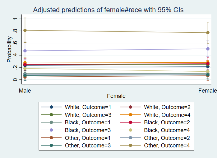
Running out of degrees of freedom is not an uncommon problem in multinomial models run on complex survey data. In the example above, we were not able to calculate the multi-degree-of-freedom test of the interaction. In other situations, when we include the interaction term, we do not get an F-statistic or a p-value for the overall model.
Again, the issue is caused by the degrees of freedom. You might think that because we have so many observations in this dataset that we could run a model with many predictors and not run out of degrees of freedom, but that is not the case. A great explanation of the problem can be found in the Stata j_robustsingular help file that you can access by clicking on the blue in the Stata output or by typing help j_robustsingular in the Stata command window.
In some analyses, the F-statistic for the overall model may not be calculated; however, the parameters are still estimated correctly. The standard errors should be carefully considered. The theory justifying the calculation of the standard errors assumes a large number of clusters minus strata. If the standard errors are suspect, then so are the test statistics and their p-values.
Count Models
Both Poisson and negative binomial models can be used with complex survey data. We will start with a simple Poisson model with a single binary predictor. We will then investigate the plausibility that the conditional variance is approximately equal to the condition mean. For more information regarding Poisson models, please see Stata Data Analysis Examples: Poisson Regression and Stata Annotated Output: Poisson Regression. For more information regarding negative binomial models, please see Stata Data Analysis Examples: Negative Binomial Regression and Stata Annotated Output: Negative Binomial Regression.
svy: poisson hdresult i.female
(running poisson on estimation sample)

Survey: Poisson regression

Number of strata = 31                             Number of obs   =      8,708
Number of PSUs   = 60                             Population size = 98,606,432
                                                  Design df       =         29
                                                  F(1, 29)        =     506.37
                                                  Prob > F        =     0.0000

------------------------------------------------------------------------------
             |             Linearized
    hdresult | Coefficient  std. err.      t    P>|t|     [95% conf. interval]
-------------+----------------------------------------------------------------
      female |
     Female  |   .1713176   .0076132    22.50   0.000     .1557469    .1868883
       _cons |   3.810654   .0085857   443.84   0.000     3.793094    3.828214
------------------------------------------------------------------------------
Note: Strata with single sampling unit centered at overall mean.

quietly svy: mean hdresult, over(female)

estat sd, var

-------------------------------------
        Over |       Mean    Variance
-------------+-----------------------
  c.hdresult@|
      female |
       Male  |   45.17997    153.0132
     Female  |   53.62264    215.3385
-------------------------------------
It seems that we have overdispersion, which is quite common in count models. Let’s try a negative binomial model. Notice that no test of the alpha parameter being equal to 0 is given, as it is when this analysis is run with unweighted data.
svy: nbreg hdresult i.female
(running nbreg on estimation sample)

Survey: Negative binomial regression

Number of strata = 31                             Number of obs   =      8,708
Number of PSUs   = 60                             Population size = 98,606,432
                                                  Design df       =         29
                                                  F(1, 29)        =     506.37
Dispersion: mean                                  Prob > F        =     0.0000

------------------------------------------------------------------------------
             |             Linearized
    hdresult | Coefficient  std. err.      t    P>|t|     [95% conf. interval]
-------------+----------------------------------------------------------------
      female |
     Female  |   .1713176   .0076132    22.50   0.000     .1557469    .1868883
       _cons |   3.810654   .0085857   443.84   0.000     3.793094    3.828214
-------------+----------------------------------------------------------------
    /lnalpha |  -3.008826   .0276271                      -3.06533   -2.952322
-------------+----------------------------------------------------------------
       alpha |   .0493496   .0013634                      .0466385    .0522183
------------------------------------------------------------------------------
Note: Strata with single sampling unit centered at overall mean.

margins female, vce(unconditional)

Adjusted predictions

Number of strata = 31                             Number of obs   =      8,708
Number of PSUs   = 60                             Population size = 98,606,432
                                                  Design df       =         29

Expression: Predicted number of events, predict()

------------------------------------------------------------------------------
             |             Linearized
             |     Margin   std. err.      t    P>|t|     [95% conf. interval]
-------------+----------------------------------------------------------------
      female |
       Male  |   45.17997   .3879036   116.47   0.000     44.38662    45.97332
     Female  |   53.62264   .4392396   122.08   0.000      52.7243    54.52099
------------------------------------------------------------------------------
Let’s try including an interaction between female and age.
svy: nbreg hdresult i.female##c.age
(running nbreg on estimation sample)

Survey: Negative binomial regression

Number of strata = 31                             Number of obs   =      8,708
Number of PSUs   = 60                             Population size = 98,606,432
                                                  Design df       =         29
                                                  F(3, 27)        =     199.91
Dispersion: mean                                  Prob > F        =     0.0000

------------------------------------------------------------------------------
             |             Linearized
    hdresult | Coefficient  std. err.      t    P>|t|     [95% conf. interval]
-------------+----------------------------------------------------------------
      female |
     Female  |    .131853   .0185006     7.13   0.000      .094015     .169691
         age |  -.0000729   .0003018    -0.24   0.811    -.0006902    .0005445
             |
female#c.age |
     Female  |   .0009366   .0003886     2.41   0.022      .000142    .0017313
             |
       _cons |   3.813683   .0154928   246.16   0.000     3.781996    3.845369
-------------+----------------------------------------------------------------
    /lnalpha |   -3.01082   .0273982                     -3.066855   -2.954784
-------------+----------------------------------------------------------------
       alpha |   .0492513   .0013494                      .0465674    .0520899
------------------------------------------------------------------------------
Note: Strata with single sampling unit centered at overall mean.
We can use the margins command to get the predicted counts.
margins female, at(age=(20(10)60)) vce(unconditional)

Adjusted predictions

Number of strata = 31                             Number of obs   =      8,708
Number of PSUs   = 60                             Population size = 98,606,432
                                                  Design df       =         29

Expression: Predicted number of events, predict()
1._at: age = 20
2._at: age = 30
3._at: age = 40
4._at: age = 50
5._at: age = 60

------------------------------------------------------------------------------
             |             Linearized
             |     Margin   std. err.      t    P>|t|     [95% conf. interval]
-------------+----------------------------------------------------------------
  _at#female |
     1#Male  |   45.25103   .4971356    91.02   0.000     44.23427    46.26779
   1#Female  |     52.605   .5194601   101.27   0.000     51.54258    53.66741
     2#Male  |   45.21807   .4250519   106.38   0.000     44.34874     46.0874
   2#Female  |   53.06136   .4554657   116.50   0.000     52.12983    53.99289
     3#Male  |   45.18514   .3893427   116.05   0.000     44.38884    45.98143
   3#Female  |   53.52167   .4379633   122.21   0.000     52.62594    54.41741
     4#Male  |   45.15223    .399671   112.97   0.000     44.33481    45.96965
   4#Female  |   53.98598   .4747944   113.70   0.000     53.01492    54.95705
     5#Male  |   45.11934   .4527185    99.66   0.000     44.19343    46.04525
   5#Female  |   54.45432   .5575775    97.66   0.000     53.31395     55.5947
------------------------------------------------------------------------------

marginsplot

But wait! There are even more commands that we have not yet covered?!?!
Yes, it is true! There are even more commands that respect the svy prefix that we have not covered. To see a full list of all of the estimation commands that respect the svy prefix, please see https://www.stata.com/manuals/svy.pdf . You will notice that the tabulate oneway and tabulate twoway commands are not included on this page; they are documented elsewhere because they are not estimation commands.
For more information on using the NHANES data sets
There are helpful resources for learning how to analyze the NHANES data sets correctly. One is a listserv at
http://www.cdc.gov/nchs/nhanes/nhanes_listserv.htm . There are
also online tutorials at
http://www.cdc.gov/nchs/tutorials/index.htm .
References
Applied Survey Data Analysis, Second Edition by Steven G. Heeringa, Brady T. West, and Patricia A. Berglund
A survey
of survey statistics: What is done and can be done in Stata by Frauke
Kreuter and Richard Valliant, The Stata Journal (2007), Volume 7,
Number 1, pages 1-21.
Goodness-of-fit test for a logistic regression model fitted using survey sample
data by Kellie J. Archer and Stanley Lemeshow, The Stata Journal (2006),
Volume 6, Number 1, pages 97-105.
Analysis of Health Surveys by
Edward L. Korn and Barry I. Graubard
Sampling of Populations: Methods
and Applications, Fourth Edition by Paul Levy and Stanley Lemeshow
Analysis of Survey Data Edited by R. L. Chambers and C. J. Skinner
Sampling Techniques, Third Edition by William G. Cochran
Stata 18 Manual: Survey Data
StatNews #73: Overlapping Confidence Intervals and Statistical Significance, October 2008 by the Cornell Statistical Consulting Unit
Why Overlapping Confidence Intervals Mean Nothing about Statistical Significance