Statistical Computing Workshop: Using the SPSS Mixed Command
PowerPoint slides: Using the SPSS Mixed Command Part 1 and Using the SPSS Mixed Command Part 2
Introduction
The purpose of this workshop is to show the use of the mixed command in SPSS. Although it has many uses, the mixed command is most commonly used for running linear mixed effects models (i.e., models that have both fixed and random effects). Such models are often called multilevel models. Because the purpose of this workshop is to show the use of the mixed command, rather than to teach about multilevel models in general, many topics important to multilevel modeling will be mentioned but not discussed in detail. References will be provided so that those interested in these topics can find additional information. The mixed command in SPSS is used to run linear regression models, including mixed effects models.
When most people think of linear regression, they think of ordinary least squares (OLS) regression. In this type of regression, the outcome variable is continuous, and the predictor variables can be continuous, categorical, or both. How would you run a linear regression model in SPSS? Perhaps you would use either the regression command or the glm command.
regression
/dep = write
/method = enter read female.
glm write with read female
/print = parameter.
Here is the same model run with the mixed command.
mixed write with read female
/fixed read female
/print = solution.
The SPSS keyword with is used with both the glm and the mixed commands to indicate that the two predictor variables, read and female, are to be treated as continuous. The print subcommand is used to have the parameter estimates included in the output (although the options used on the subcommand are different).
Obviously, there are already several ways to run an OLS regression in SPSS, so what else can the mixed command do? It can run linear models with clustered data. Remember that one of the most important assumptions of OLS regression is that the observations are independent. From a practical stand point, this means that each observation is represented on one and only one row in the data file. The effects of violating this assumption depend on the extent to which the assumption is violated. If this assumption is violated by having clustering in the data, the point estimates, standard errors and degrees of freedom will be estimated incorrectly. Please see Harrell (2015) and Scariano and Davenport (1987) for explanations and examples.
Repeated measures
How do data become clustered? One way is to collect data on the same subjects over time. For example, a researcher might measure subjects’ blood pressure at three different time points. Let’s take a moment to look at our example data set. We have the outcome at three time points and two categorical predictors, diet (diet) and exercise type (exertype). Because multiple observations are made on the same subjects, each data point is related to all of the other data points collected from that subject. Technically, we say that the errors within subjects are correlated. Because the observations are not independent, we cannot use the regression command, or the standard errors will be biased, and hence, the test statistics an p-values will be inaccurate. So what procedure can be used? A common choice is the glm command with the wsfactor subcommand. We are going to start with an example of repeated measures ANOVA because, like OLS regression, most researchers are familiar with this type of analysis. In order to use the glm command for a repeated measures ANOVA, the data must be structured in wide format.
data list free / id exertype diet time1 time2 time3.
begin data.
1     1         1       85       85       88
2     1         1       90       92       93
3     1         1       97       97       94
4     1         1       80       82       83
5     1         1       91       92       91
6     1         2       83       83       84
7     1         2       87       88       90
8     1         2       92       94       95
9     1         2       97       99       96
10    1         2      100       97      100
11    2         1       86       86       84
12    2         1       93      103      104
13    2         1       90       92       93
14    2         1       95       96      100
15    2         1       89       96       95
16    2         2       84       86       89
17    2         2      103      109       90
18    2         2       92       96      101
19    2         2       97       98      100
20    2         2      102      104      103
21    3         1       93       98      110
22    3         1       98      104      112
23    3         1       98      105       99
24    3         1       87      132      120
25    3         1       94      110      116
26    3         2       95      126      143
27    3         2      100      126      140
28    3         2      103      124      140
29    3         2       94      135      130
30    3         2       99      111      150
end data.
Let’s say that the hypothesis to be tested is that diet affects blood pressure. Blood pressure readings from three times are contained in the variables time1, time2 and time3. The glm syntax for this would be:
glm time1 time2 time3 by diet
/wsfactor = time 3
/wsdesign = time
/design = diet.
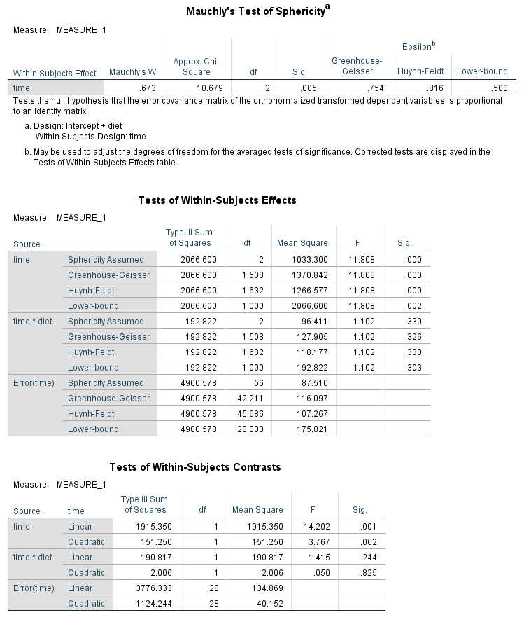
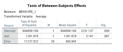
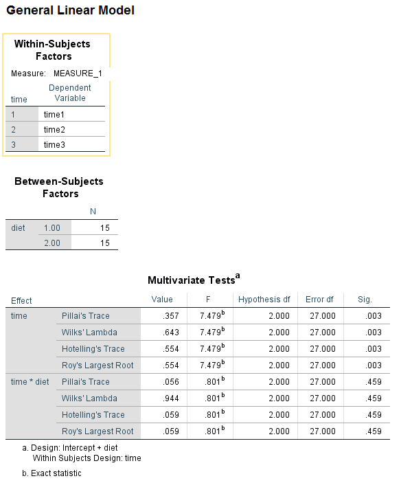
We can see that time is statistically significant, but diet and the time by diet interaction is not. Wait a minute – time by diet interaction? Where did we specify that in our glm syntax? An interaction of the variable listed on the wsfactor subcommand and the predictor variable(s) is included in the model by default, at least for the multivariate tests. From the SPSS documentation for the GLM: Repeated Measures entry we learn:
“A repeated measures analysis includes a within-subjects design describing the model to be tested with the within-subjects factors, as well as the usual between-subjects design describing the effects to be tested with between-subjects factors. The default for the within-subjects factors design is a full factorial model which includes the main within-subjects factor effects and all their interaction effects.”
For some analyses, this may be appropriate, but what if you don’t want this interaction in model? The answer is that you must use a different command, because there is no way to override this default.
Relationship between time points
Now let’s think about the relationship between these repeated observations. We know that they are not independent, but how, exactly, are they related? We could imagine that the relationship was the same across time, so that it was either set to a specific constant (such as 0) or estimated as a single value. At the other extreme, we could assume that every value needed to estimated. Another possibility is that the relationship between the time points decreases as the distance between the time points increases; in other words, time points that are close together are more closely related than time points that are further apart.
       time1   time2   time3
time1

time2

time3
So what did SPSS use? For the univariate results, SPSS used compound symmetry (CS). This structure estimates one value for the variances and another value for the covariances. For the mulitivariate results an unstructured (UN) covariance structure was used, meaning that every value in the variance-covariance matrix was estimated. These defaults are used by all statistical software packages for repeated measures analyses. This is default that cannot be altered in the glm command, even if it does not do a good job of representing the data.
Missing data
Let’s consider one more important point about these data.
id exertype diet time1 time2 time3

1 1 1 85 85 88
2 1 1 90 92 93
3 1 1 97 97 94
4 1 1 80 82 83
5 1 1 91 92 91
....
What if we had been unable to measure S3’s blood pressure at time 3? Now suppose that we were also unable to measure S2’s blood pressure at time 1? SPSS (and all other general-use statistical software) uses listwise deletion by default. This means that even a little bit of missing data could be a big problem. Another limitation of the repeated measures ANOVA analysis is that all of the predictors must be at the level of the person; we cannot include any predictors that vary by time (Harrell, 2015).
Reshaping the data from wide to long
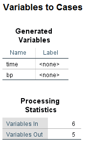
Since this is a a workshop on the SPSS mixed command, let’s find out how the mixed command can help us out with these issues. We will start by running our model with the mixed command. Before we can do that, however, we will first need to restructure the data. The glm command requires the data to be in wide form, but mixed command requires the data to be in long form. We can use the varstocases command to restructure the data from wide to long.
varstocases
/make bp from time1 time2 time3
/index = time.
To be clear on what just happened, let’s look at the data before and after the restructuring:
Data in wide form
id exertype diet time1 time2 time3

1 1 1 85 85 88
2 1 1 90 92 93
3 1 1 97 97 94
4 1 1 80 82 83
5 1 1 91 92 91
Data in long form
id exertype diet time bp

1 1 1 1 85
1 1 1 2 85
1 1 1 3 88
2 1 1 1 90
2 1 1 2 92
2 1 1 3 93
3 1 1 1 97
3 1 1 2 97
3 1 1 3 94
4 1 1 1 80
4 1 1 2 82
4 1 1 3 83
5 1 1 1 91
5 1 1 2 92
5 1 1 3 91
Data in wide format are also known as multivariate, because there are multiple dependent variables (DVs). Data in long format are also known as univariate, because there is a single DV. So we have gone from having the DV spread across multiple columns to having the DV in a single column.
An example using the mixed command with the repeated subcommand
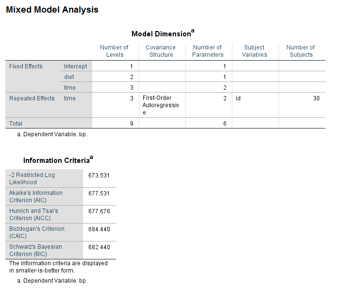
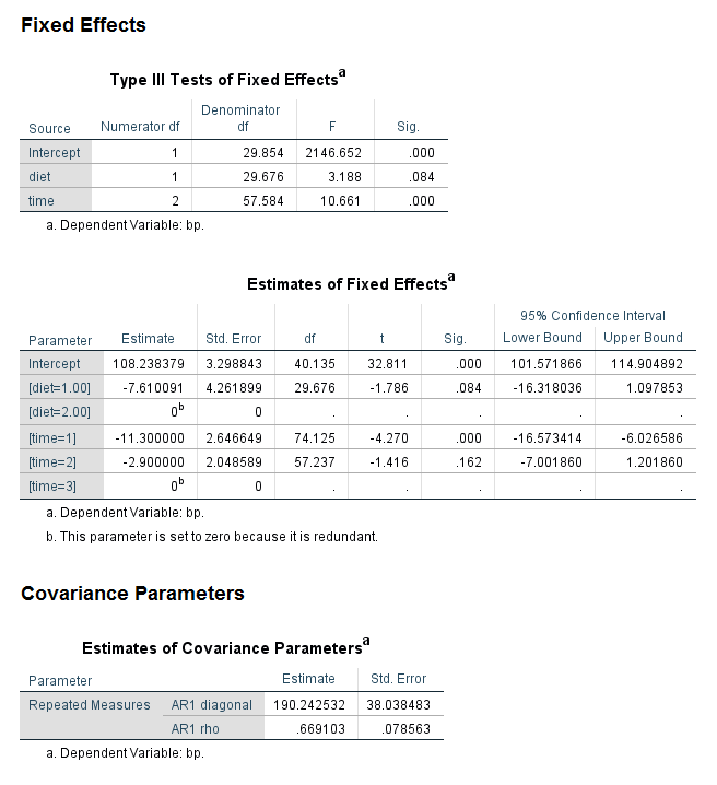
Now let’s get back to the mixed command, using, of course, the data in long format. Now it is easy to exclude unwanted interaction terms by simply not including them on the fixed subcommand. We can change the covariance structure by altering the structure given in the covtype option on the repeated subcommand.
mixed bp by time diet
/fixed diet time
/repeated time | subject(id) covtype(ar1)
/print = solution.
How are missing data handled? Listwise deletion is still used, but the effect on the analysis is different.
id exertype diet time bp

1 1 1 1 85
1 1 1 2 85
1 1 1 3 88
2 1 1 1 90
2 1 1 2 92
2 1 1 3 93
3 1 1 1 97
3 1 1 2 97
3 1 1 3 94
4 1 1 1 80
4 1 1 2 82
4 1 1 3 83
5 1 1 1 91
5 1 1 2 92
5 1 1 3 91
Even if datum from one time point is missing, the data from the other time points are still included in the analysis. This illustrates an important point: Subjects do not need to have the same number of observations. In other words, subjects can have different numbers of rows of data. As we will see in some examples a little later on in this workshop, adding time-varying predictors variables is as simple as listing them on the mixed command and on the fixed subcommand.
Let’s consider two more important points before leaving this analysis. First, with a repeated measures ANOVA, the time points are to be equally spaced. Secondly, everyone is to be measured at those exact times. In our example, subjects’ blood pressure was measured at 15 minute intervals. In carefully controlled experiments, this isn’t usually a problem. In other research situation, however, this isn’t feasible. Mixed effects models do not require that subjects be measured at the same intervals.
The take-away message is not that repeated measures ANOVAs are bad or flawed, but rather that repeated measures ANOVAs are a limited set of multilevel models. Indeed, mixed effect analyses are themselves a limited case of another type of analysis. On page 145 of Harrell (2015), there is a very nice table that lists the different ways that repeated measures data can be analyzed and notes the features and limitations of each of these options.
Clustered data
Let’s return to the question of how data might be clustered and consider another example. Instead of observations clustered within a person, we could have people clustered in families, patients clustered in hospitals or students clustered in classrooms. In our next example dataset, we will have students clustered, or nested, in classrooms. We will use the hsbdemo dataset in our examples. The variable cid is the classroom identifier, and the variable id is the student identifier.
Let’s look at the first 15 observations for some of the variables that will be used in the upcoming examples.
sort cases by cid id.

list cid id write read female prog
/cases from 1 to 15.

cid  id write read female prog

  1   1   44   34     1     3
  1   2   41   39     1     3
  1  15   39   39     0     3
  1  45   35   34     1     3
  1  51   36   42     1     1
  1  53   37   34     0     3
  1  67   37   37     0     3
  1 108   33   34     0     1
  1 133   31   50     0     3
  1 153   31   39     0     3
  1 164   36   31     0     3
  2  11   46   34     0     2
  2  16   31   47     0     3
  2  19   46   28     1     1
  2  89   35   35     1     3


Number of cases read:  15    Number of cases listed:  15
An example of mixed without accounting for clustering
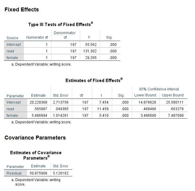
Suppose we wanted to build a linear regression model regressing write on read and female. Here is the mixed syntax to do that. (This is the same OLS regression model from earlier in the workshop.)
mixed write with read female
/fixed read female
/print = solution.
Looking at the section of the output called Fixed Effects, we see two tables. The first table, the Type III Tests of Fixed Effects, gives the overall statistical significance for each of the predictors in the model. Because both of the predictors in our model have only one degree of freedom, this information is redundant with the information in the next table. However, if we had included categorical predictor variables in our model that had more than two levels, this table would be very useful, because it would give the multi-degree-of-freedom test of the those variables. We will see an example of this later on in this workshop. The table called Estimates of Fixed Effects gives the coefficients, standard errors, degrees of freedom, test statistic, significance, and lower and upper confidence intervals for the predictors. It is usually the table that everyone hurries to once they have run a model. In this output, we can see that both read and female are statistically significant predictors. The coefficients, listed in the column called Estimates, are interpreted just like coefficients from an OLS regression. For example, for a one-unit increase in read, the expected value of write increases by 0.565887 unit. In the section of the output called Covariance Parameters, we see the estimate of the residual, which is 50.875908.
An example of the mixed command accounting for clustering
Now let’s run this same model but account for the clustering of students in classrooms. One new subcommand has been added to account for the clustering of students in classrooms, the random subcommand. The SPSS keyword intercept has been included on this subcommand to specify a random intercept model. This type of model is commonly used to account for clustering in data.
Let’s mention a few important points before we actually run the model. First, the lowest level of a multilevel model is called level 1. The outcome variable must be at level 1. A multilevel model must have at least two levels, and in our example here, the model only has two levels, so level 2 is the highest level. Predictor variables can be at any level of the model, and SPSS (and almost all statistical software packages) will automatically detect the level of each predictor; there is no need to provide that information. How does the software detect the level of each variable? If the variable changes within the level 2 identifier, then it is a level 1 variable. If the variable is constant within the level 2 identifier, then it is a level 2 variable. This means that all multilevel datasets must have a level 2 identifier (and an identifier for all levels above level 2, if there are any).
mixed write with read female
/fixed read female
/random intercept | subject(cid)
/print = solution.
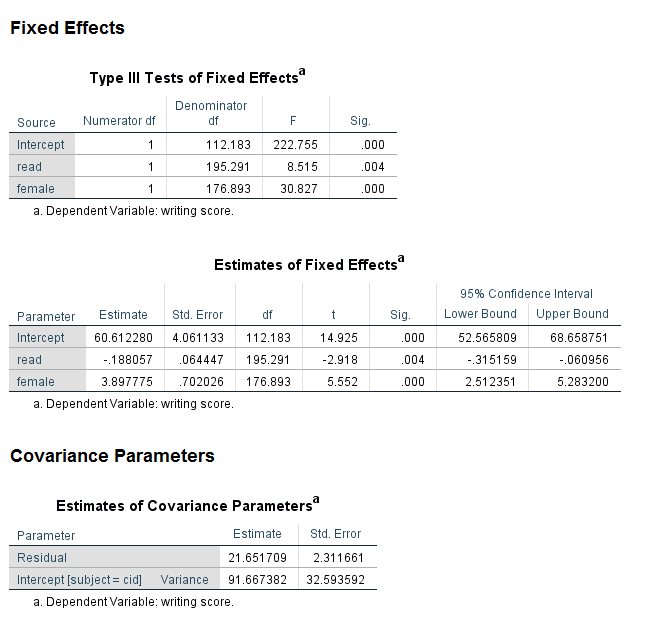
The first thing to notice is that the point estimates, their standard errors, and the degrees-of-freedom are very different in this analysis compared to the analysis that did not account for the clustering. In other words, accounting for the clustering (AKA non-independence) is very important. Note that the same level 2 identifier, in our example, the variable cid, would be used in every analysis. The clustering is a feature of the data that does not change, so it is always included in the analysis and in the same way.
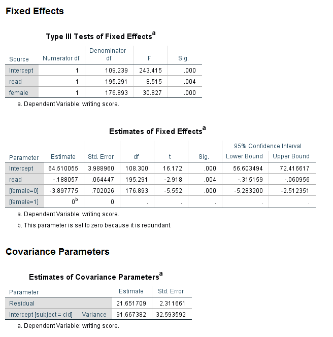
Let’s look at the section of the output called Fixed Effects. As before, we can see in the table called Type III Tests of Fixed Effects that both read and female are statistically significant, although the F values are different. Looking at the table called Estimates of Fixed Effects, we can see that the coefficients are very different. The coefficient for read is now negative, such that for a one-unit increase in read, the expected value of write decreases by 0.188057.
Looking at the section called Covariance Parameters, we can see that another line is included in the table called Estimates of Covariance Parameter. The estimate of the level 1 residual is given on the first line as 21.651709. On the next line, we have the estimate of the variance around the grand intercept. The value is 91.667382. This value, like the value of the level 1 residuals, is rarely of interest and is not interpreted, although it is usually reported.
The binary variable female (0 = male, 1 = female) is treated as a continuous predictor variable in the analysis above because it is included after the SPSS keyword with, but it could be treated as a categorical variable as well. To do this, we can include it after the SPSS keyword by. When a predictor variable is specified as categorical, SPSS will by default use the highest numbered category as the reference group. This means that if a variable is coded as 0 and 1, the group coded 1 will be the reference group. Hence, the sign of the coefficient for the binary predictor will be different when it follows the SPSS keyword with than when it follows the SPSS keyword by. The intercept will also be different. There is no way to change the reference group of a categorical predictor variable in the mixed command; the only way to change the reference group is to create a new variable with the categories ordered differently. If this is needed, be certain to label the new variable and its values very carefully, so that there is no confusion with the original variable.
mixed write with read by female
/fixed read female
/random intercept | subject(cid)
/print = solution.
Notice that the values in the table called Type III Tests of Fixed Effects are the same as in the previous analysis. However, the coefficients for the intercept and female are different, although the coefficient for read is the same. The last line of the table is for female = 1, and the coefficient is 0. The footnote reminds us why: “The parameter is set to 0 because it is redundant.” In other words, for a categorical predictor variable with only two levels, there can be only one coefficient. The fact that the estimated coefficient is for female = 0 reminds us that the reference group for female is 1, rather than 0. The values in the table called Estimates of Covariance Parameters are the same as the previous analysis.
When a predictor variable is specified as categorical, it can also be specified on the emmeans subcommand. The emmeans subcommand is used to get estimated marginal means, which can be thought of as a type of descriptive statistic that is based on the model. Estimated marginal means can help researchers better understand their results.
mixed write with read by female
/fixed read female
/random intercept | subject(cid)
/print = solution
/emmeans = tables(female).
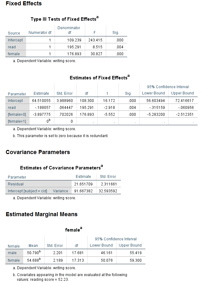
Notice that the parameter for female = 0 is -3.89775. Now look at the values in the table called Estimated Marginal Means at the end of the output. The mean for males is 50.790 and the mean for females is 54.688. What value do you get if you subtract the mean for the females from the mean for the males? We have seen that binary predictor variables can be modeled as either continuous or categorical, but how should one choose which way to model such variables? In some sense, it does not really matter, because the models are equivalent. Notice that for both models, the -2 restricted log likelihood is 1253.994 and, in fact, all of the information in the table Information Criteria is exactly the same. This is also true of the table Type III Tests of Fixed Effects and the table Estimates of Covariance Parameters. To be clear, there is no “right” or “wrong” way to model a binary predictor: either way is OK. The decision on how to model a binary predictor (as continuous or categorical) in SPSS should depend on which group you want to have as the reference group and whether or not the variable is needed on the emmeans subcommand.
Adding more predictors
Now let’s add another continuous predictor, socst, and another categorical predictor, prog, to the model. Notice that the SPSS keywords with and by are only specified once each; all of the continuous predictors are listed after the SPSS keyword with and all of the categorical predictor variables are listed after the SPSS keyword by. It does not matter if with or by is specified first, only that they are specified only once, if specified at all. Notice also that more than one emmeans subcommand can be specified.
mixed write with read socst by female prog
/fixed read socst female prog
/random intercept | subject(cid)
/print = solution
/emmeans = tables(female)
/emmeans = tables(prog).
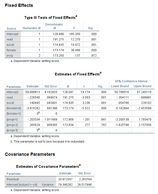
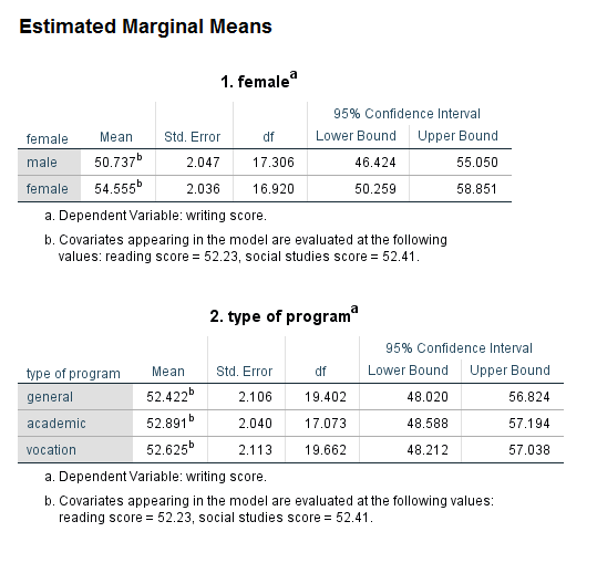
Looking at the table called Type III Tests of Fixed Effects, we can can see that all of the predictor variables are statistically significant except for prog. Notice that the test of prog has two degrees of freedom (because the variable prog has three levels). In the table called Estimates of Fixed Effects we find the coefficients, and, as expected, the coefficient for the highest-numbered category of female and prog are 0 (because they are the reference groups). At the bottom of the output, there are two tables of Estimated Marginal Means. Looking at the table for prog, we can see that the estimated marginal mean for each level of prog is approximately 52. This fact can help us (and audience members) understand why prog is not a statistically significant predictor.
Random slopes
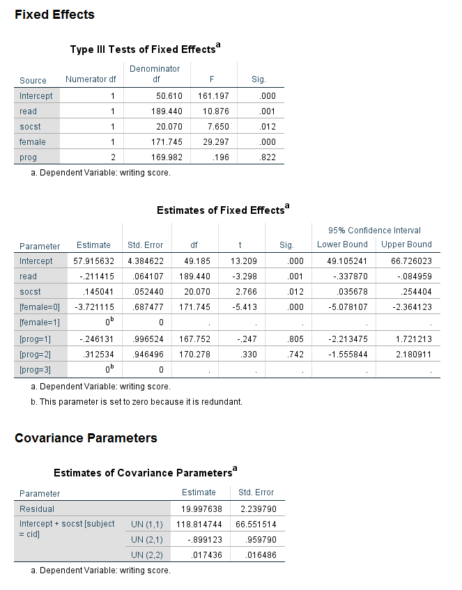
Another way that this model can be extended is by including a random slope. The inclusion of a random slope in a multilevel model should be done only when theory indicates the random slope is necessary or when testing a specific hypothesis. The random intercept is almost always included in a multilevel model, as it accounts for the clustering in the data; the random slope, on the other hand, is often optional. When a random slope is included, the random intercept and random slope might covary, in which case a covariance structure should be specified. If a covariance structure is not specified using the covtype option on the random subcommand, SPSS will use variance components (VC) by default. In the next example, the variable socst will be included on the random subcommand and an unstructured variance structure (UN) will be specified. The specification of the covtype option can be shortened to just cov.
mixed write with read socst by female prog
/fixed read socst female prog
/random intercept socst | subject(cid) cov(un)
/print = solution.
The tables in the Fixed Effects part of the output look as we expect; the new information is in the table called Estimates of Covariance Parameters at the bottom of the output. The first line in the table gives the estimate and standard error of the level 1 residual. The second line gives the estimate of the variance and its standard error for the random intercept. The third line gives the covariance between the random intercept and the random slope and its standard error. We can see that this estimate is negative, meaning that higher the random intercept, the less steep the slope is. Conversely, the lower the intercept, the more steep the slope is. In the last line, the estimate of the variance around the random slope is given, along with its standard error. Clearly, there is much more variance around the grand intercept than around the grand slope. While the value of the variance around the random slope does not need to be interpreted, if it is very close to 0, it may be better to omit the random slope from the model.
Watch for error messages
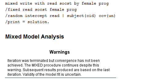
Random slopes sometimes cause estimation problems, and not all models with random slopes will converge, as we see in the next example. Be careful to look for error messages in the output file immediately after the echo of the syntax, as SPSS will often provide the results from the last iteration, even if there was a problem with the estimation.
mixed write with read socst by female prog
/fixed read socst female prog
/random intercept read | subject(cid) cov(un)
/print = solution.
Choosing between the repeated and random subcommands
In the example using repeated measures data, the repeated subcommand was used to specify the repeated measures. However, the random subcommand could also have been used. One of differences between the repeated and random subcommands is what covaries. When the repeated subcommand is used, the covariance structure specifies the covariance between the time points. When the random subcommand is used, the covariance is between the random intercept and the random slope or slopes.
Tests of random effects
It seems reasonable to ask if these random effects are statistically significant. In fact, SPSS does offer a testcov option on the print subcommand that will provide such a test. However, not all statisticians believe that this is a valid test. The problem with this type of test is that the null hypothesis (namely that the random effect equals 0) is on the boundary of the parameter space. Please see Parameter Estimation and Inference in the Linear Mixed Model by N. N. Gumedze and T. T. Dunne (2011) for more information. The solution option can also be added to the random subcommand to include the random effects parameter estimates.
Choosing a covariance structure
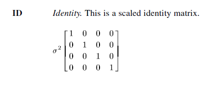
When running a model that has both a random intercept and a random slope, there is a covariance between the random intercept and the random slope. The default in SPSS is to use variance components (VC). When the variance components structure is specified on a random subcommand, a scaled identity (ID) structure is assigned to each of the effects specified on the subcommand. A scaled identity matrix has 1s on the diagonal (for the variances), and 0s on the off-diagonal (for the covariances). For many research situations, this is unrealistic, so a different type of covariance structure may be specified. Below are some examples of commonly used covariance matrices.
Identity
Compound symmetry
First order autoregressive
Heterogeneous first order autoregressive
Unstructured
Chapters 7 and 8 of Applied Longitudinal Data Analysis by Singer and Willett (2003) provide excellent descriptions and explanations of the issues.
Comparing models with different covariance structures
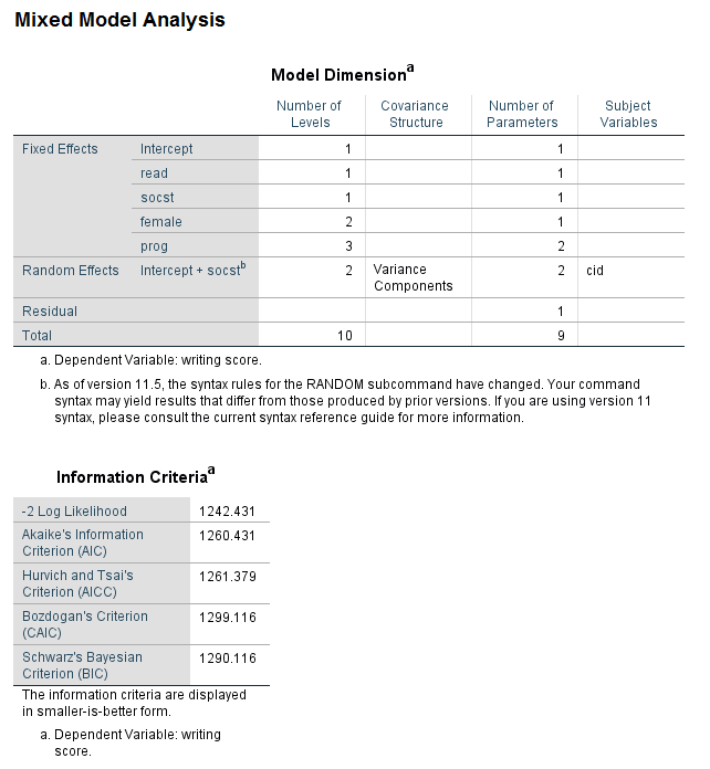
In some research situations it is clear which covariance structure should be used. In other research situations, however, the researcher may wish to test models that use different covariance structures to determine which is preferable. A likelihood ratio test (LRT), also known as a likelihood ratio chi-square test, is sometimes used for this purpose. By default, the SPSS mixed command uses restricted maximum likelihood (REML). While a likelihood ratio chi-square can be calculated with REML in some circumstances, it is not always appropriate. We are not going into this issue here, but you can get more information on this issue here: Full ML v. Restricted ML. For the example below, we will include the method subcommand with the ml option to change from the default to maximum likelihood.
* -2 log likelihood = 1242.431, number of parameters = 9.
mixed write with read socst by female prog
/fixed read socst female prog
/random intercept socst | subject(cid) cov(vc)
/method = ml
/print = solution.
* -2 log likelihood = 1241.234, number of parameters = 10.
mixed write with read socst by female prog
/fixed read socst female prog
/random intercept socst | subject(cid) cov(un)
/method = ml
/print = solution.
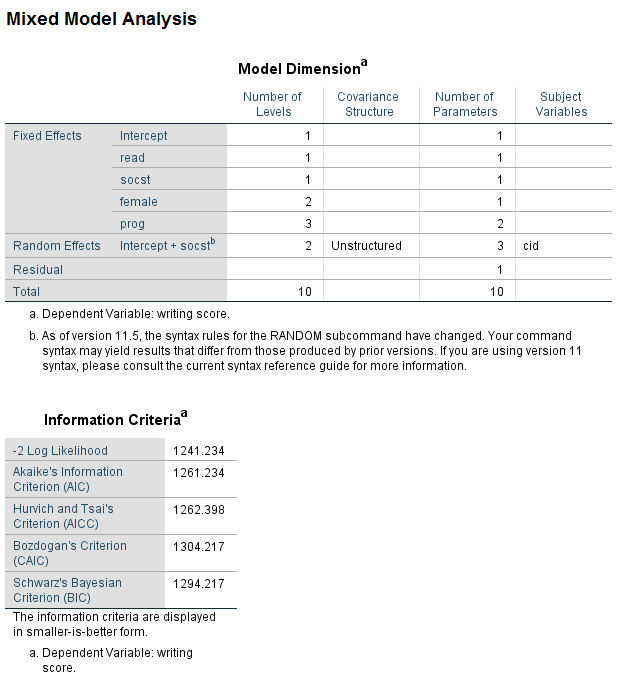
The likelihood ratio test is easily calculated by hand. To do this, note the -2 log likelihood and the number of parameters from each model. In this example, the difference in -2 log likelihoods is very small (approximately 1.2), and the difference in degrees of freedom is 1. The critical value for a chi-square test with one degree of freedom is 3.841, which is well above our observed value of 1.2; hence, we conclude that the difference between the models is not statistically significant. Given this, the model with the variance components covariance is to be preferred. It should be acknowledged that not all statisticians believe that this is the best way to determine which covariance structure is best for a given model . Chuck Kincaid gives a description of various methods that can be used to choose between covariance structures (Guidelines for Selecting the Covariance Structure in Mixed Model Analysis )
As a final note, here is a webpage with useful information on when to use and when not to use an unstructured covariance structure: The Unstructured Covariance Matrix: When It Does and Doesn’t Work. The likelihood ratio chi-square works only when models are nested. In the example above, the models are nested because we are comparing a model using variance components to a model with an unstructured covariance structure. This test would not be valid if we compared the model with variance components to a model using AR1. When comparing models that are not nested, values such as AICC or BIC are often examined. With these types of measures, the model with the smaller value is to be preferred. However, caution should be used so that the model is not overfit to the data. A good discussion of the different types of information criteria and their limitations can be found in The Comparison of Model Selection Criteria When Selecting Among Competing Hierarchical Linear Models. Keselman, Algina, Kowalchuk and Wolfinger (A Comparison of Two Approaches For Selecting Covariance Structures in The Analysis of Repeated Measurements ) describe the limitations of using AIC or BIC when selecting models with different covariance structures.
ML v. REML
Even if you are not comparing models, you may still wonder whether to use ML or REML. REML is often preferred when the sample size is small (Raudenbush and Bryk, 2002). With these types of measures, the model with the smaller value is to be preferred. However, caution should be used so that the model is not overfit to the data. However, many sources that make this recommendation do not clearly state what is meant by “small”. The default in SPSS is to use REML, but this can be changed by using the ML option on the method subcommand.
Confidence intervals and denominator degrees of freedom
There are many options available on the criteria subcommand. The cin option allows you to specify confidence level desired; the default is 95%. You can also change the method used to calculate the denominator degrees of freedom. There are three methods available: Satterthwaite, residual and kenwardroger. Please see the SPSS Command Syntax Reference Guide for a complete description of these options. Briefly, Satterthwaite is often used when the sample size is small (however the term “small” is defined), the data are unbalanced, and/or a complicated covariance structure is used (e.g., an unstructured covariance matrix). A different value for the denominator degrees of freedom may be used across the different tests shown in the output, and the value may include a decimal (AKA, the value of the denominator degrees of freedom may not be a whole number). With the residual option, a single value is used for the denominator degrees of freedom across all tests. This option may be preferable when the sample size is large, the data are balanced, and/or a simple covariance matrix is used. The kenwardroger option may be preferable when the sample size is small; it provides a an approximation of the degrees of freedom with t-tests and F-tests. All of these options adjust both the confidence intervals and the p-values.
There are several other options available on the criteria subcommand. These options govern the process of model convergence, but they are usually best left at their default values. It is important to verify that your model converged before you start interpreting your results. By default, SPSS will display the results as of the last iteration of the model even if the model did not converge. If this happens, a warning message will be shown at the beginning of the output, but you may need to scroll up in the output window to see it.
Disaggregating level 1 and level 2 effects
While multilevel models can have predictors at any level of the model, the interpretation of the coefficients is more straight forward when the predictors are at level 2 (or the highest level of the model). This is because the values within each cluster are constant, and therefore the effect can only be at that level. When a predictor level is measured at level 1, then the values change not only within cluster but between clusters as well. In other words, the effect of the predictor on the outcome happens at both level 1 and level 2. If there is only a single coefficient for this predictor in your output, then it is necessarily some combination of the effect at level 1 and level 2. It is usually desirable to disaggregate the effect of the predictor into its level 1 effect and level 2 effect. A common way to do this is to create an aggregated variable (AKA a level 2 variable) from the level 1 variable. The SPSS command aggregate can be used for this purpose. However, a few cautions are in order. Research has shown that creating a level 2 variable by aggregated data collected at level 1 may lead to a point estimate that is attenuated (meaning smaller than it should be), and the standard error may also be too small. Please see Lüdtke, et. al. (2008) and Schunck (2016) for more information and possible solutions. Despite these concerns, we will show the SPSS syntax for aggregating the level 1 predictor to create a level 2 predictor. We will use the predictor variable read for our example.
aggregate
/break = cid
/mread = mean(read).
We will also center the level 2 predictor.
means var = read.
compute cread = read - 52.23.
execute.

mixed write with mread cread
/fixed mread cread
/random intercept | subject(cid)
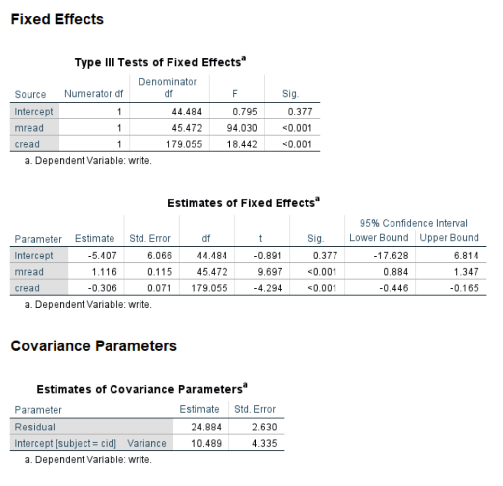
/print = solution.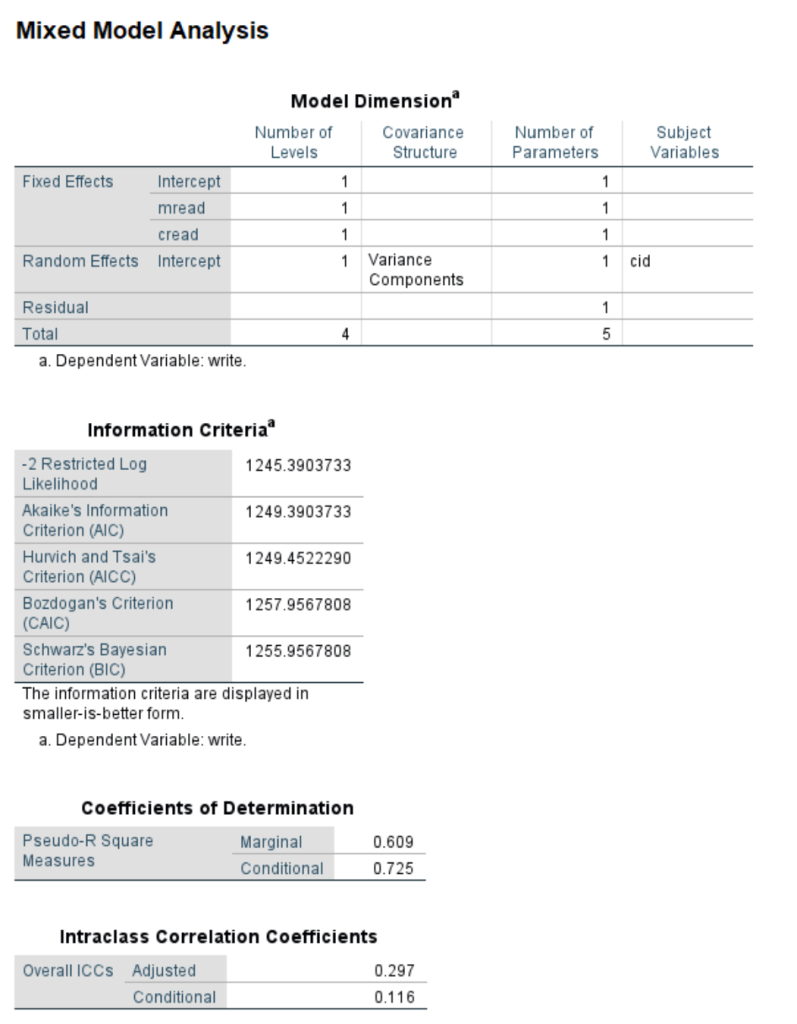
Interactions
Now let’s talk about interactions. Multilevel models can include interaction terms, just as any other regression model can. The terms included in the interaction may be at level 1 or level 2 (or any higher level if the multilevel model has more than two levels). The terms in the interaction do not have to be at the same level. When the terms are not at the same level, the interaction is called a cross-level interaction. The example dataset does not have a level 2 predictor variable, so one will be created for the purpose of the following example analysis. The first sort cases command is necessary for the aggregate command to work correctly; the second is simply to put the data back in the order they were before the new variable was created – it is technically not necessary.
sort cases by cid honors.

aggregate
/break = cid
/sum_honors = sum(honors).

sort cases by cid id.
exe.
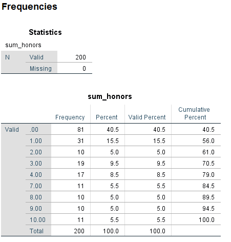
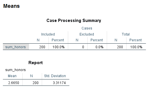
Let’s get some descriptive statistics on the new variable, sum_honors.
freq var = sum_honors.
means var = sum_honors.
The variable sum_honors is ordinal, so it could be used as either a categorical or a continuous predictor variable, depending on our research purpose.
In our first example, we include an interaction of two level 1 variables. Because both of the variables are categorical, they are both listed after the SPSS keyword by on the mixed command. The specification of the interaction term is given on fixed subcommand.
mixed write by female prog
/fixed female prog female*prog
/random intercept | subject(cid)
/print = solution
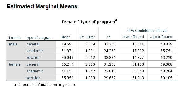
/emmeans = tables(female*prog).
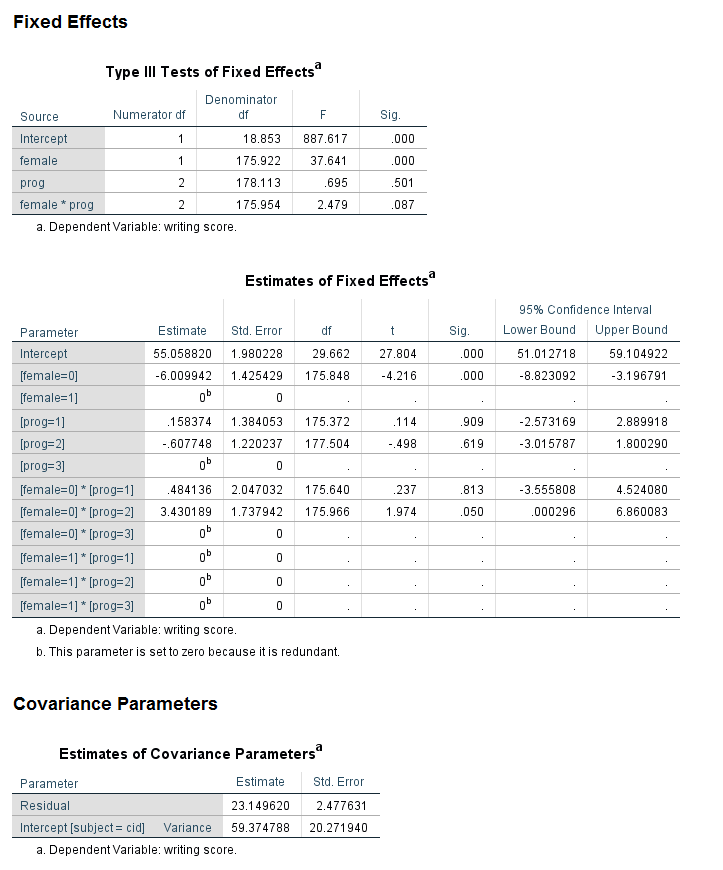
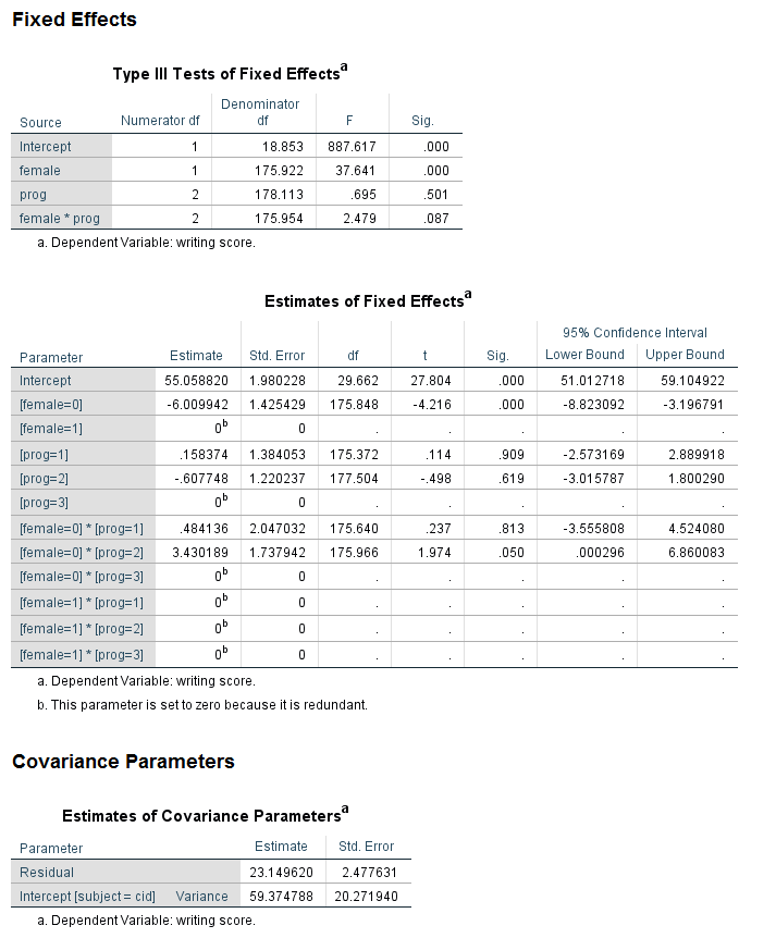
Looking at the table called the Type III Tests of Fixed Effects, we can see that the predictor variable female is statistically significant, while prog and the female by prog interaction are not. Looking at the table called the Estimates of Fixed Effects, we see that neither of the coefficients for the variable prog are statistically significant, so this is consistent with the output in the table above. Looking at the interaction term, the coefficient for the female = 0 by prog = 1 term is not statistically significant, but the coefficient for female = 0 by prog = 2 has a p-value of 0.05, and the lower bound of the confidence interval does not include 0 (although it is very close). While some researchers might try to interpret this coefficient, most would not because the overall test of the interaction was not statistically significant.
Interaction of a level 1 and level 2 predictor
Now let’s interact the level 2 predictor variable sum_honors with a level 1 predictor variable, female.
mixed write by female sum_honors
/fixed female sum_honors female*sum_honors
/random intercept | subject(cid)
/print = solution
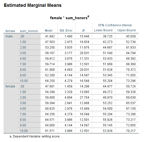
/emmeans = tables(female*sum_honors).
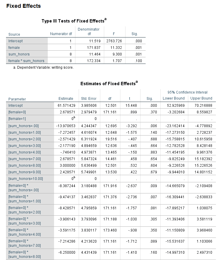
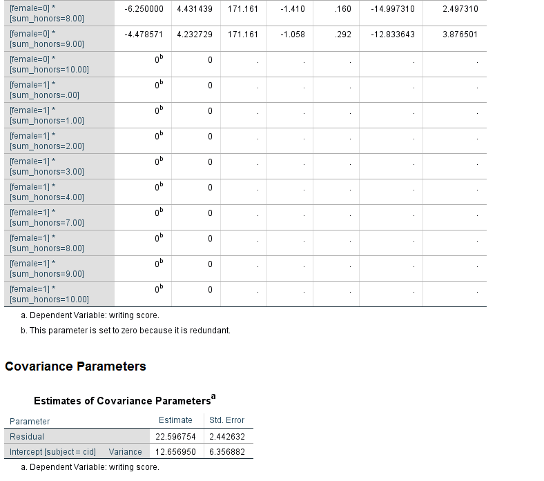
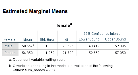
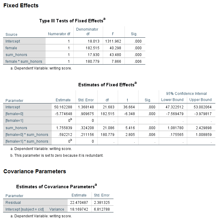
Looking at the table called Type III Tests of Fixed Effects, we can see that the interaction of female and sum_honors is not statistically significant. Looking at the table called Estimates of Fixed Effects, we see that two coefficients in the interaction term are statistically significant; again, this would not be interpreted because the overall interaction term (the 8 df test) is not statistically significant. Comparing the results for the variable female in the table of Type III Tests of Fixed Effects and the Estimates of Fixed Effects, we see that in the former table, the p-value for female is 0.001, while in the latter table the p-value is 0.370. Why are these p-values so different? The difference is caused by the type of coding scheme used for the categorical variables. In the table of Type III Tests of Fixed Effects, effect coding is used for the categorical variable. However, in the table of Estimates of Fixed Effects, dummy coding is used. This difference matters only when there is an interaction term in the model and one or more of the variables in the interaction is categorical. The p-value of the interaction term is not affected, but the p-values of the lower-order terms may be. Oftentimes, the lower-order effects are not interpreted (although they are always reported), so the difference is of minimal consequence. It is not the case that one p-value is correct and the other is not; rather, they give different information. When reporting the results, it is important to be clear which is being reported. The results in the table Type III Tests of Fixed Effects are main effects, while the results in the table estimates of Fixed Effects are simple effects. Main effects are deviations from the grand mean, while simple effects are the effect at a specific value. For these results, we would say that the effect of being male compared to female is 2.678571 at the reference level of prog and the reference level of the interaction term. This test may or may not be of interest to the researcher. While the coefficients and their p-values are always reported, the simple effect may or may not be interpreted.
The variable sum_honors is ordinal, so it is possible to treat it as continuous. In the following example, sum_honors is treated as a continuous predictor. On the emmeans subcommand, it has been held at its mean, which is 2.665 (rounded to 2.67).
mixed write by female with sum_honors
/fixed female sum_honors female*sum_honors
/random intercept | subject(cid)
/print = solution
/emmeans = tables(female) with (sum_honors = 2.67).
In this model, the interaction as well as both of the lower-order effects, is statistically significant.
Tests of simple main effects
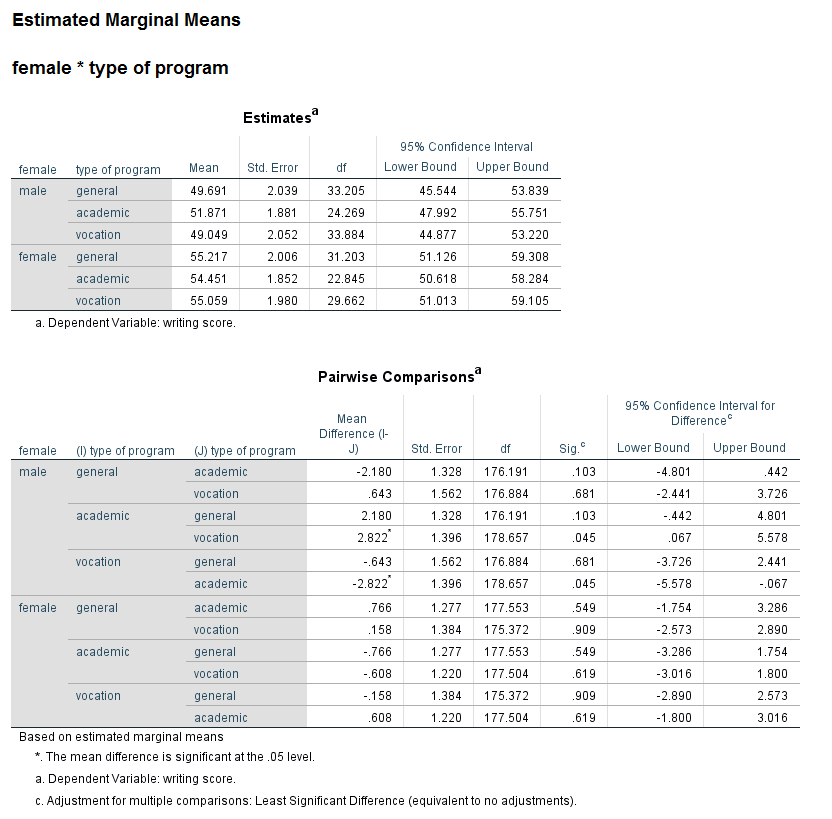
When there is an interaction in the model, a test of simple main effects is sometimes useful. A test of simple main effects asks if the effect of one variable is statistically significant at a given level of another variable. This test can be obtained by using the compare option on the emmeans subcommand. Let’s return to the earlier example that included the interaction of the two level 1 variables female and prog.
mixed write by female prog
/fixed female prog female*prog
/random intercept | subject(cid)
/print = solution
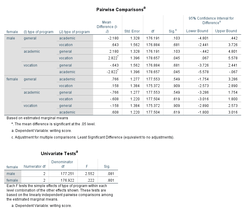
/emmeans = tables(female*prog) compare(prog).
Be aware that not all statisticians approve of the use of tests of simple main effects. In particular, there are concerns over the conceptual error rate. Tests of simple main effects are one tool that can be useful in interpreting interactions. Caution should be exercised in interpreting the results of analyses of simple main effects. In general, the results of tests of simple main effects should be considered suggestive and not definitive.
More options on the emmeans subcommand
There are several useful option on the emmeans subcommand, and they should be used when they are useful. Be aware that they can add a good deal of extra output, so using only what will be useful to you in your current research situation is a good idea. Some of the options are shown in the following examples.
mixed write by female prog with read
/fixed female prog female*prog read
/random intercept | subject(cid)
/print = solution
/emmeans = tables(female*prog) with(read = mean) compare(prog) adj(bonferroni).

mixed write by female prog with read
/fixed female prog female*prog read
/random intercept | subject(cid)
/print = solution
/emmeans = tables(female*prog) with(read = mean) compare(prog) refcat(last) adj(bonferroni).
Testing custom hypotheses
Let’s look at a few examples of the test subcommand. The test subcommand is used to test custom hypotheses. Specifically, you specify the null hypothesis as a linear combinations of parameters. You can use multiple test subcommands in a given call to mixed and each is treated independently. Multiple linear combinations can also be specified on a single test subcommand, and when this is done, they need to be separated with a semicolon. The contrast coefficients listed on the test subcommand should always sum to 0. In our first example, we will use effect coding to test the effect of the variable female. As a side note, the code below is actually the multilevel version of a t-test.
mixed write by female
/fixed female
/random intercept | subject(cid)
/print = solution
/emmeans = tables(female)
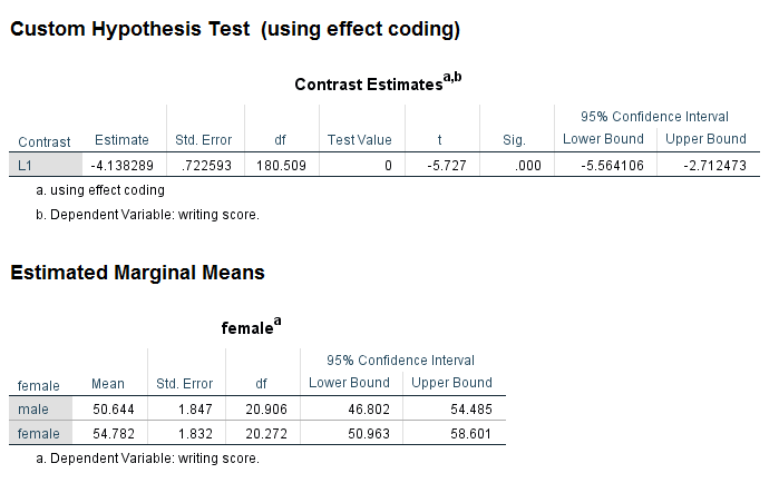
/test = 'using effect coding' female 1 -1.
We can see the results in the section of the output called Custom Hypothesis Test in the table called Contrast Estimates. The contrast estimate is -4.138. The output from the emmeans subcommand shows the estimated marginal means for each level of female. Because we used effect coding, the contrast coefficient is the difference between these two means.
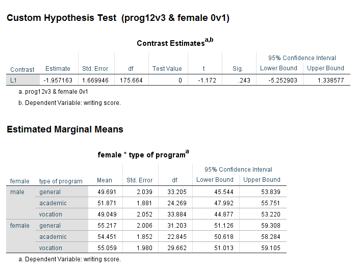
Interaction contrasts can be done using the test subcommand. Let’s say that we want to compare the average program type 1 and 2 versus 3 and female 0 versus 1. Before trying to write the syntax, let’s make a table with the two categorical predictor variables, female and prog, along with the values of the contrast coefficients.
              prog 1 = -.5 prog 2 = -.5 prog 3 = 1

female 0 =  1        -.5       -.5         1
female 1 = -1         .5        .5        -1
mixed write by female prog
/fixed female prog female*prog
/random intercept | subject(cid)
/print = solution
/emmeans = tables(female*prog)
/test = 'prog12v3 & female 0v1' prog*female -.5 -.5 1 .5 .5 -1.
We can see the results in the table called Contrast Estimates. None of the three contrasts that were specified are statistically significant.
In the next example, multiple linear combinations will be specified on a single test subcommand. The variable prog, which has three levels, will be used. The first will compare level 1 of prog with level 3; the second will compare level 1 with level 2; and the third will compare level 2 with level 3. This is done only to show an example of how to use the divisor option.
mixed write by prog
/fixed prog
/random intercept | subject(cid)
/print = solution
/emmeans = tables(prog)
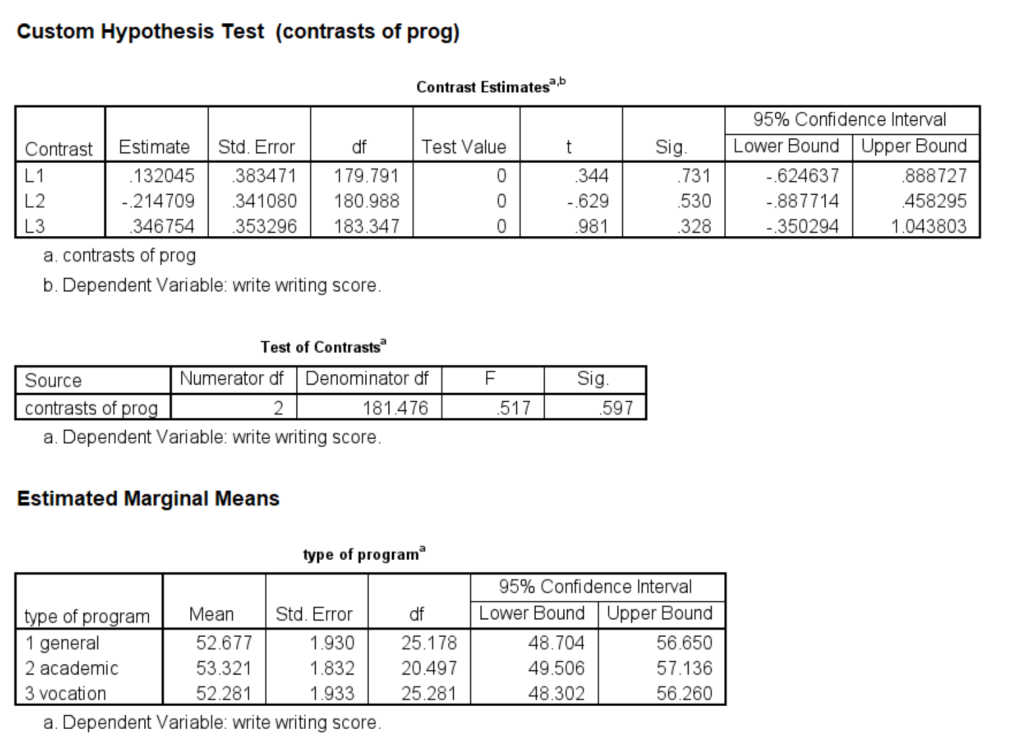
/test = 'contrasts of prog' prog 1 0 -1 divisor = 3; prog 1 -1 0 divisor = 3; prog 0 1 -1 divisor = 3.
The 1 degree of freedom tests are shown in the table Contrast Estimates; the 2 degree of freedom test is given in the table called Tests of Contrasts. We can see that none of these tests are statistically significant.
Adding more output
The print subcommand can be used to include more output if desired. Some useful options include the following, the descriptions of which are quoted directly from the SPSS Command Syntax Reference Guide:
corb: Asymptotic correlation matrix of the fixed-effects parameter estimates
covb: Asymptotic covariance matrix of the fixed-effects parameter estimates
CPS: Case Processing Summary – Displays the sorted values of the factors, the repeated measure variables, the repeated measure subjects, the random-effects subjects, and their frequencies
descriptives: Displays the sample sizes, the means, and the standard deviations of the dependent variable, and covariates (if specified). These statistics are displayed for each distinct combination of the factors
g: Estimated covariance matrix of random effects. This keyword is accepted only when at least one RANDOM subcommand is specified. Otherwise, it will be ignored. If a SUBJECT variable is specified for a random effect, then the common block is displayed
history: Iteration history – The table contains the log-likelihood function value and parameter estimates for every n iterations beginning with the 0th iteration (the initial estimates). The default is to print every iteration (n = 1). If HISTORY is specified, the last iteration is always printed regardless of the value of n
lmatrix: Estimable functions – Displays the estimable functions used for testing the fixed effects and for testing the custom hypothesis
R: Estimated covariance matrix of residual – This keyword is accepted only when a REPEATED subcommand is specified. Otherwise, it will be ignored. If a SUBJECT variable is specified, the common block is displayed
solution: A solution for the fixed-effects parameters. The fixed-effects parameter estimates are displayed. Their approximate standard errors are also displayed
covtest: Tests for the covariance parameters – Displays the asymptotic standard errors and Wald tests for the covariance parameters
Saving variables to the active dataset
The save subcommand can be used to save any of seven different variables related to the current multilevel model to the active dataset. To do this, the temporary variable name must be specified on the save subcommand, and an optional new name can be specified in parentheses. In the following example, five new variables will be saved to the dataset. These are the fixed predicted values, which are the regression means without the random effects (called blue); the predicted values, which are the model fitted values (called blup); the standard error of the fixed predicted values (called seblue); the standard errors of the predicted values (called seblup); and the level 1 residuals (called resid1).
mixed write with read socst by female prog
/fixed read socst female prog
/random intercept socst | subject(cid) cov(un)
/print = solution
/save = fixpred(blue) pred(blup) sefixp(seblue) sepred(seblup) resid (resid1).

list cid id write blue blup seblue seblup resid1
/cases from 1 to 10.
cid id write blue blup seblue seblup resid1

 1 1 44 56.67 40.42 2.35 1.47 3.58
 1 2 41 55.62 39.37 2.23 1.46 1.63
 1 15 39 52.04 35.80 2.26 1.44 3.20
 1 45 35 54.50 38.11 2.58 1.96 -3.11
 1 51 36 54.45 38.18 2.22 1.64 -2.18
 1 53 37 51.50 35.16 2.51 1.60 1.84
 1 67 37 51.01 34.68 2.42 1.53 2.32
 1 108 33 51.98 35.68 2.46 1.62 -2.68
 1 133 31 48.12 31.77 2.30 1.77 -.77
 1 153 31 53.35 37.19 2.24 1.99 -6.19


Number of cases read: 10 Number of cases listed: 10
The acronym BLUP stands for best linear unbiased prediction, and it is used in linear mixed models for the estimation of random effect. It is similar to the best linear unbiased estimates (BLUEs) of fixed effects. Please see That BLUP is a good thing: The estimation of random effects for more information.
If you change the model but not the names of the variables to be saved to the dataset, you will get an error message indicating that the variable names given on the save subcommand name variables already in the dataset. You can use the delete variables command to remove the variables from the dataset.
delete variables blue blup seblue seblup resid1.
mixed write with read by female
/fixed read female
/random intercept socst | subject(cid) cov(un)
/print = solution
/save = fixpred(blue) pred(blup) sefixp(seblue) sepred(seblup) resid(resid1).
Amount of variance explained
As was made clear earlier in this workshop, the SPSS mixed command is used to run linear models, models that are, in many ways, similar to OLS regression. The R-squared value associated with an OLS model is often used to describe the amount of variance in the outcome variable that is explained by the predictor variables. Unfortunately, there is no obvious equivalent in a multilevel model. However, there are some approximations that can be calculated. There are good discussions of this topic Snijders and Bosker (2012), chapter 7 and Singer and Willett (2003) pages 102-104. A currently preferred method has been proposed by Rights and Sterba (2018).
Checking model assumptions
For the most part, the assumptions of OLS regression also apply to linear multilevel models. However, most of the assumptions apply to each level of the multilevel model.
1. Independence of observations This assumption applies only at the highest level of nesting. Also, it is assumed that no important level of nesting is omitted from the model. If a level of nesting is omitted, the variance associated with that level will be mainly distributed to the level immediately below, as well as the level immediately above, if there is a level above (Snijder and Bosker, 2012).
2. Correct specification of the model This means that all of the necessary variables are specified for both the fixed and random parts of the model for each level of the model. It also means that no unnecessary variables are included.
3. Functional form The predictors are linearly related to the outcome. To test this assumption at level 1, a graph would be made for each level 2 unit of the outcome and each predictor. To test this assumption at level 2, plots of OLS estimates against each level 2 predictor would be made.
4. Homoscedascity The residuals have a constant variance. Heteroscedascity may be observed if an important variable is omitted from the model. To test this assumption, plots of the raw residuals against each predictor would be made. 5. Normality of residuals All residuals in the model are normally distributed. Many researchers, including Singer and Willett (2003, page 128) prefer visual inspection of such graphs rather than formal tests such as Wilks-Shapiro or Kolmogorov-Smirnov.
Checking the assumptions of even a simple multilevel model is a lot of work. For the first two assumptions, it is up to the researcher to know these things about the data and the model. The other two assumptions can be assessed with graphs. We will take a very simple model as an example. The save subcommand will be used to save the necessary variables to the dataset.
* checking model assumptions.
mixed write with read
/fixed read
/random intercept  | subject(cid)
/print = solution
/save = fixpred(blue_read) pred(blup_read) resid(resid1_read).
** Output omitted.
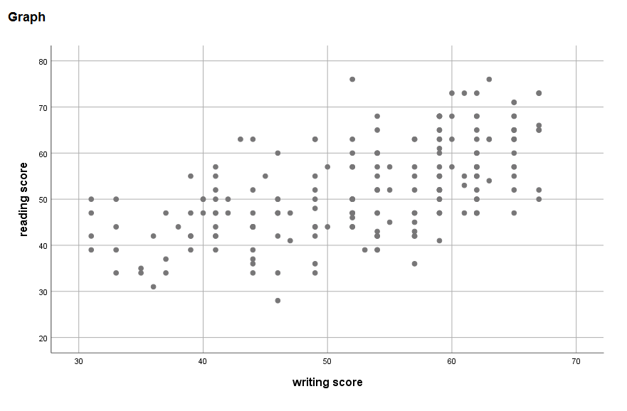
* linearity.
graph
/scatterplot write with read.
The relationship between write and read appears to be mostly linear.
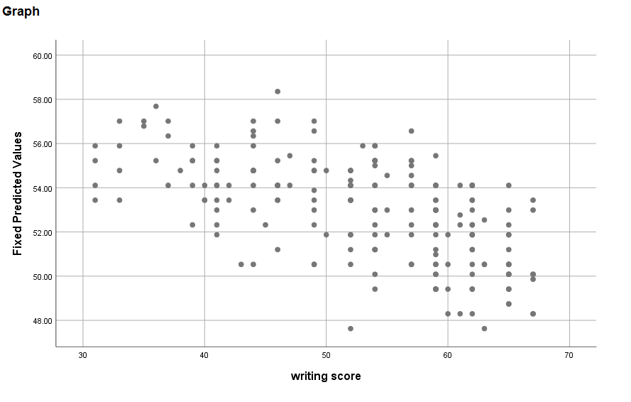
* homogeneity.
graph
/scatterplot write with blue_read.
The variance seems to be smaller at lower values of write.
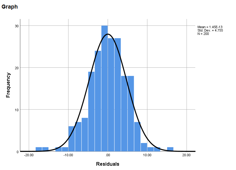
* normality.
graph
/histogram(normal) = resid1_read.
The residuals appear to be approximately normally distributed.
An example of a three-level model
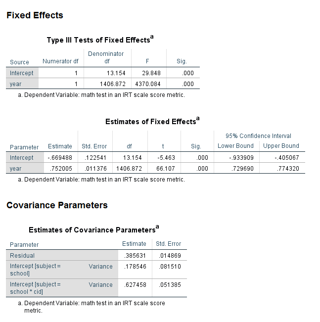
Let’s look at an example of a three-level model. In this example, we have students nested within classrooms nested within schools. Notice that two random subcommands are needed. The first specifies the highest level of the model, and the second specifies the second-highest level nested in the highest level. This example can be expanded to run models with four, five or even more levels. The dataset eg_hlm_small is used here.
mixed math with year
/fixed = year
/print = solution
/random = intercept | subject(school)
/random = intercept | subject(school*cid).
Other topics
For this last section, let’s discuss some common issues regarding multilevel models.
Intraclass correlation
As we know, the observations within clusters are not independent. We can assess the extent of the non-independence of observations within clusters by calculating the intraclass correlation. To do this, we run a null model (i.e., a model with no predictor variables, which can also be called an empty model, and intercept-only model or an unconditional means model) and then do a little simple math by hand. We will use the hsbdemo dataset that we used before for this example. First, the formula:
The numerator is the between-cluster variance, and the denominator is the sum of the between-cluster and within-cluster variance. The SPSS syntax needed to get these two numbers is minimal.
mixed write
/random intercept | subject(cid).
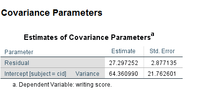
Looking at the table called Estimates of Covariance Parameters at the bottom of the output, we can see that the between-cluster variance is 64.361 and the within-cluster variance is 27.297. Hence, the ICC is 0.70. Values of ICC can range from 0 to 1, so a value of .7 is fairly large. Reporting an ICC value is often a requirement of peer-reviewed journals. Please note that there are at least 10 different definitions of ICC, so when reporting an ICC, you need to be clear about which version of ICC you are reporting. Please see A guideline of selecting and reporting intraclass correlation coefficients for reliability research for more information.
Design effect
Another reason to calculate an ICC is to determine if the non-independence in the data is “strong” enough to warrant the use of a multilevel model. If the data are nearly independent and all of the variables in the model are at the same level, a single-level model would be preferred because it is more parsimonious. To determine if a multilevel model is really needed, the design effect can be calculated. Again, this is a simple formula with math that can be done by hand.
design effect = 1 + (average_cluster_size – 1)*ICC
The ICC can be calculated as shown above. The average cluster size can be found with the use of the aggregate command.
aggregate outfile = "D:\data\temp\mixed_n.sav"
/break = cid
/num_cid = nu(cid).

get file "D:\data\temp\mixed_n.sav".
mean num_cid.
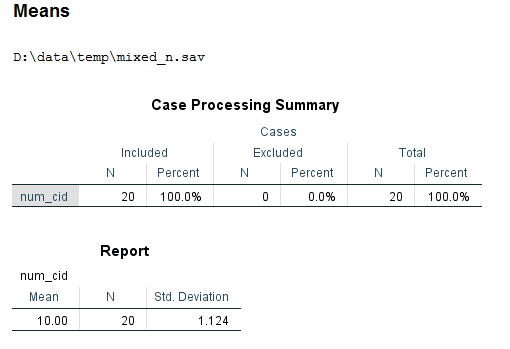
We can see that the average cluster size is 10.00. So, design effect = 1 + (10 – 1)*.7 = 7.3 If the design effect is less than 2 (Muthen and Satorra, 1995), we can safely ignore the clustering in the data. In this example, the design effect is much greater than 2, so a multilevel model (or some other method) is needed to account for the clustering in the data.
Denominator degrees of freedom
There is more than one way to calculate the denominator degrees of freedom in a multilevel model. Prior to SPSS version 26, the only option for the calculation of the denominator degrees of freedom was the Satterthwaite approximation This method is valid for both balanced and unbalanced designs. Starting with SPSS version 27, other option are residual and kenwoodroger.
Centering
Centering is a big topic that will not be covered in detail in this workshop. For those not familiar with the term centering, “centering” means subtracting a mean from each value of a variable. Level 1 variables can be centered around their group means or the grand mean; level 2 variables can be grand-mean centered. In times past, centering was almost expected. Currently, it is suggested that centering be used with caution and good reason. There are references at the end of with workshop that provide further information. Please note that statistical thinking regarding centering has evolved over time, so it may be important to note the publication date of references. Please see HLM centering and Centering or not centering in multilevel models? The role of the group mean and the assessment of group effects for more information.
Sample size
The final topic is that sample size, and one of the most common questions regarding sample size is “how small is too small?”. One widely-cited article by Cora Mass and Joop Hox from 2005 has some specific recommendations based on simulations that they ran. The short summary of their findings is that about 50 level 2 observations are needed to avoid bias in the parameter estimates. Since then, many have questioned the need for 50 level 2 units, and indeed, much research using multilevel models has been published with fewer than 50 level 2 units. It is worth remembering, however, that multilevel models run on maximum likelihood, which is based on asymptotics, which necessarily requires a large sample size. Also, it is known that maximum likelihood can give biased results when run with small sample sizes; but the question of “how small is too small?” remains. Again, this is a big topic that is only being mentioned here; please see the references below for more information. If a power analysis for a multilevel model is needed, there are few off-the-shelf software packages available. One free option is: ML PowerSim . Another option is to use Optimal Design (Optimal Design ). Be aware that such power analyses usually require information that is not readily available and is not part of the standard multilevel output.
Imperfect hierarchies
In all of our previous examples, the hierarchy of observations has been very clear: each level 1 observation was clustered in one and only one level 2 unit. Not all data are so neatly structured. Imagine what our data would look like if some students started the academic year in one classroom, and then switched to another classroom at some point during the year. Now those students would be associated with more than one classroom. This is an example of a multiple membership model. With cross-classified data, each lower-level unit belongs to one higher-level unit (call it A), and also to another type of higher-level unit (call it B), but the higher-level units are not nested either way (meaning that A is not nested in B, and B is not nested in A). In multiple membership multiple classification models, both situations mentioned above are present. Chapter 13 in Snijders and Bosker (2012) gives a detailed explanation of these models, as well as examples of how to analyze such data. We do not have an example dataset to illustrate the analysis of imperfect hierarchies. Some sample syntax for a cross-classified model, taken from Multilevel Cross-Classified and Multi-Membership Models is shown below.
mixed attain with vrq
/fixed vrq
/print = solution
/random intercept | subject(pid)
/random intercept | subject(sid).
For more information on the SPSS mixed command
Please see the SPSS Command Syntax Reference for the most up-to-date information about the SPSS mixed command. You can access the Syntax Reference Guide by clicking on Help -> Command Syntax Reference.
References
De Leeuw, J. Centering in linear multilevel models. In Encyclopedia of Statistics in Behavioral Science. Everitt, B. S. and Howell, D. C., editors. volume 1, pages 247-249. http://onlinelibrary.wiley.com/doi/10.1002/0470013192.bsa085/pdf
Gumedze, F. N. and Dunne, T. T. Paramter estimation and inference in the linear mixed model. Linear Algebra and its Applications, 435(8), 1920-1944. https://www.sciencedirect.com/science/article/pii/S002437951100320X
Harrell, Jr. F. E. Regression modeling strategies with applications to linear models, logistic and ordinal regression, and survival analysis, second edition. 2015. New York: Springer.
Heck, R. H., Thomas, S. L. and Tabata, L. N. (2014). Multilevel and Longitudinal Modeling with IBM SPSS, second edition. New York: Routledge.
Hedeker, D. Multilevel cross-classified and multi-membership models https://www.ihrp.uic.edu/files/CrossClassMultiMember-Hedeker2014.pdf
http://www.unc.edu/~dbauer/manuscripts/BauerSterba_appendix_SPSS.pdf
IBM Support: Denominator degrees of freedom for fixed effects in SPSS mixed
http://www.unc.edu/~dbauer/manuscripts/BauerSterba_appendix_SPSS.pdf .
Kelly, J., Evans, M. D. R., Lowman, J. and Kykes, V. (2017). Group-mean-centering independent variables in multilevel models is dangerous. Quality and Quantity, 51(1), 261-283. https://link.springer.com/article/10.1007/s11135-015-0304-z
Kenny, D. A. and Judd, C. M. (1986). Consequences of violating the independence assumption in analysis of variance. Psychological Bulletin, 99(3), 422-431. http://psycnet.apa.org/record/1986-21031-001
Keselman, H. J., Algina, J., Kowalchuk, R. K. and Wolfinger, R. D. A comparison of two approaches for selecting covariance structures in the analysis of repeated measures. https://pdfs.semanticscholar.org/1d6c/f16816f05b6a80fa466111dea22b680f596c.pdf
Kincaid, C. Guidelines for Selecting the covariance structure in mixed model analysis. http://www2.sas.com/proceedings/sugi30/198-30.pdf
Koo, T. K. and Li, M. Y. (2016). A guideline for selecting and reporting intraclass correlation coefficients for reliability research. Journal of Chiropractic Medicine, 15(2), 155-163. https://www.ncbi.nlm.nih.gov/pmc/articles/PMC4913118/
Leyland, A. H. A review of multilevel modelling in SPSS (2004). https://www.bristol.ac.uk/media-library/sites/cmm/migrated/documents/reviewspss.pdf
Muthen, B. O. and Satorra, A. (1995). Complex sample data in structural equation modeling. Sociological Methodology, vol. 25, pages 267-316. http://www.jstor.org/stable/271070
Paccagnella, O. Centering or not centering in multilevel models? The role of the group mean and the assessment of group effects. (2006). Evaluation Review, 30(1), 66-85. https://www.ncbi.nlm.nih.gov/pubmed/16394187
Raudenbush, S. W. and Bryk, A. S. Hierarchical Linear Models: Applications and Data Analysis Methods, Second Edition. (2002). Thousand Oaks, CA: Sage Publications.
Robinson, G. K. That BUP is a good thing: The estimation of random effects. (1991). Statistical Science, 6(1), 15-2. https://projecteuclid.org/euclid.ss/1177011926
Scariano, S. M. and Davenport, J. M. The effects of violations of independence assumptions in the one-way ANOVA. (1987). The American Statistician, 41(2), 123-129. http://www.jstor.org/stable/2684223
Singer, J. D. and Willett, J. B. Applied longitudinal data analysis: Modeling change and event occurrence. 2003. New York: Oxford University Press.
Snijders, T. A. B. and Bosker, R. J. Multilevel analysis: An introduction to basic and advanced multilevel modeling, second edition. 2012. Thousand Oaks, CA: Sage Publications.
Whittaker, T. A. and Furlow, Carolyn F. (2009). The Comparison of Model Selection Criteria When Selecting Among Competing Hierarchical Linear Models. Journal of Modern Applied Statistical Methods. 8(1), 173-193. https://pdfs.semanticscholar.org/8b74/fb3018a6d65d9fdb63c1326f4fa311ed35f3.pdf
Full ML v. Restricted ML http://www.ssicentral.com/hlm/help6/faq/Full_ML_vs_Restricted_ML.pdf
The Unstructured Covariance Matrix: When It Does and Doesn’t Work https://www.theanalysisfactor.com/unstructured-covariance-matrix-when-it-does-and-doesn%E2%80%99t-work/

