About This Presentation
- It is a broad survey of count regression models
- It is designed to demonstrate the range of analyses available for count regression models
- It is not an in-depth statistical presentation
- It is not a how-to manual that will train you in count data analysisWhy Use Count Regression Models
- Count data is common in many disciplines
- Count models can be used for rate data in many instances by using exposure
- Count data often analyzed incorrectly with OLS regression
Regression Models with Count Data Outline
- Poisson Regression
- Negative Binomial Regression
- Zero-Inflated Count Models
- Zero-inflated Poisson
- Zero-inflated Negative Binomial
- Zero-Truncated Count Models
- Zero-truncated Poisson
- Zero-truncated Negative Binomial
- Hurdle Models
- Random-effects Count Models
Poisson Distribution
The Poisson probability distribution.

- λ is the mean or expected value of a Poisson distribution
- λ is also the variance of a Poisson distribution
- Poisson is a one parameter λ (lambda)
Likelihood function for the Poisson model.


Some History of the Poisson Distribution
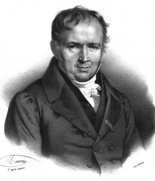
The Poisson distribution was first published by Siméon-Denis Poisson in 1838.
There is a famous example from a 1898 book by Ladislaus von Bortkiewicz showing that the number of soldiers killed by mule-kicks each year in the Prussian cavalry followed a Poisson distribution. The title of the book was The Law of Small Numbers.

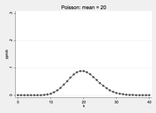
Poisson Examples
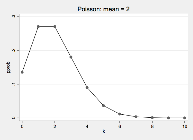
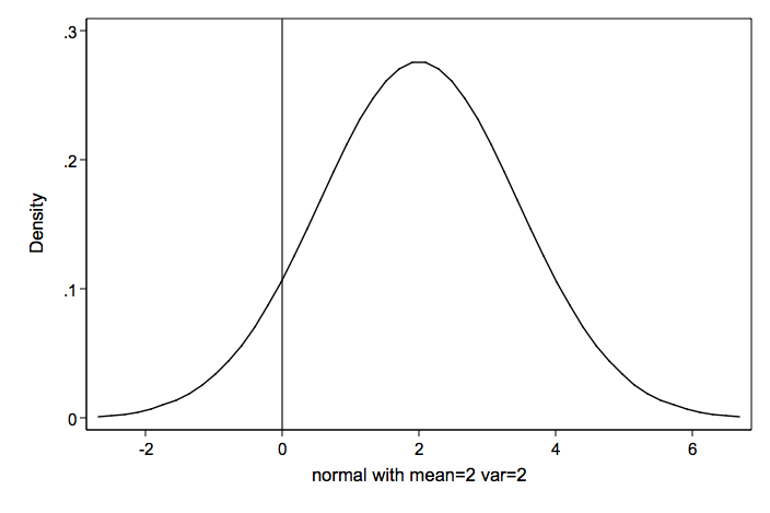
As a comparison, here is a normal distribution with the same mean and variance as the Poisson distribution above.
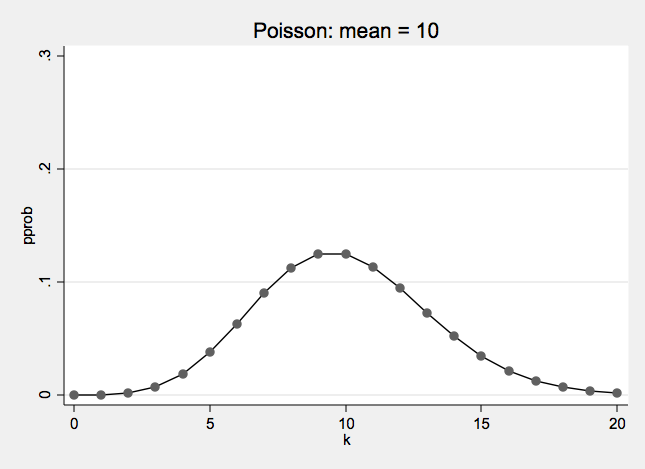
Negative Binomial Distribution One formulation of the negative binomial distribution can be used to model count data with over-dispersion.

- The negative binomial distribution has two parameters: λ and α
- λ is the mean or expected value of the distribution
- α is the over dispersion parameter
- When α = 0 the negative binomial distribution is the same as a Poisson distribution
Likelihood function for the negative binomial model.


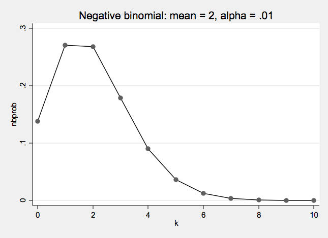
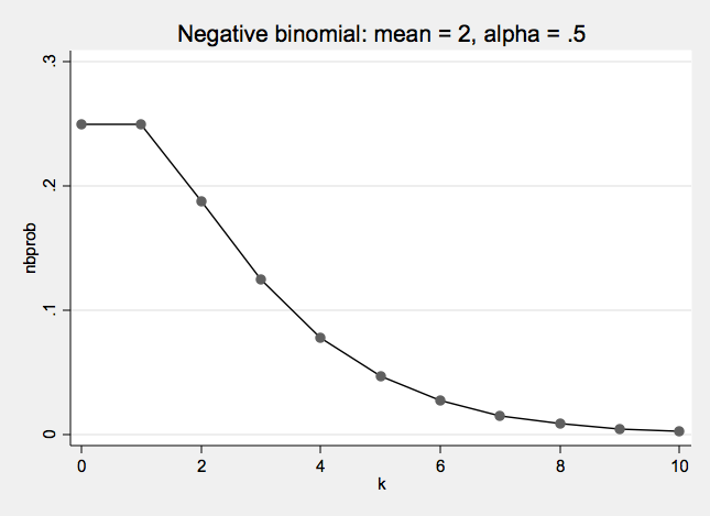
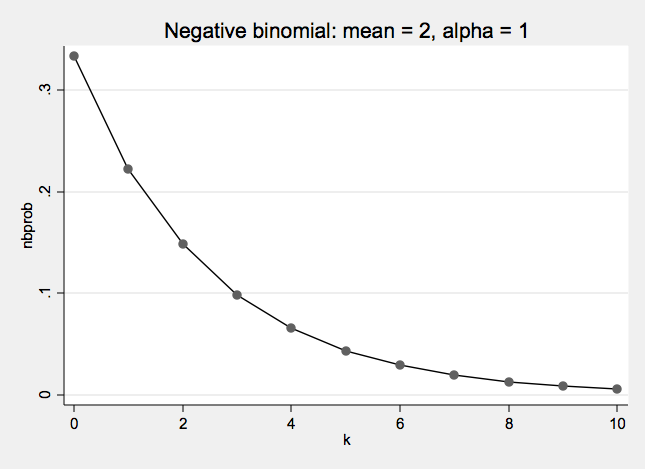
Negative Binomial Examples
Maximum Likelihood Estimation
Count models are estimated using maximum likelihood
Log likelihood:
- Computationally, the log of the likelihood function is easier to work with.
- Analysis proceeds iteratively until the log likelihood converges.
- Larger (in the closer to zero sense) log likelihoods are better.BIC:
- Schwartz’ Bayesian information criterion = -2*ln(L)+k*ln(n).
- Given any two estimated models, the model with the lower value of BIC is the one to be preferred.
- Can be used to compare different models, even models that are non-nested.
- Interpretation of absolute difference: 0-2 Weak, 2-6 Positive, 6-10 Strong, and >10 Very Strong.Sample size:
- The small sample behavior of ML estimators for count models is largely unknown.
- It is risky to use ML with samples smaller than 100.
- Samples over 500 seem adequate.
Soccer Goals Example
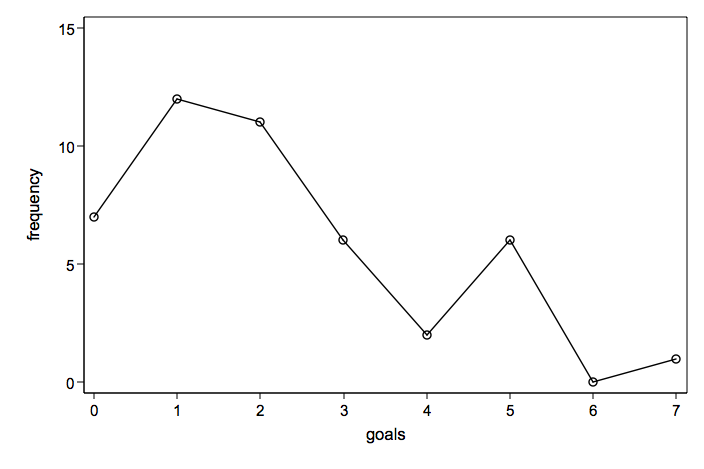
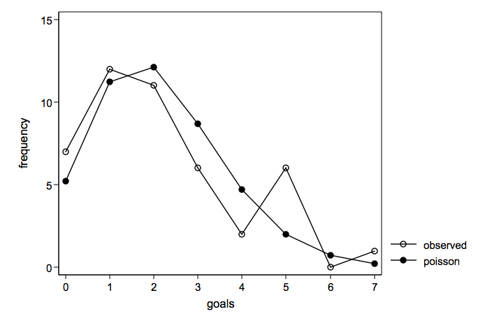
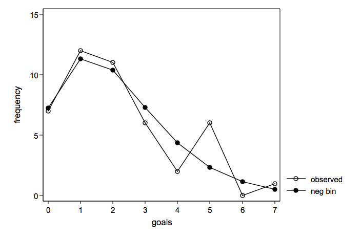
Number of goals scored for each game in a season (mean= 2.16 variance= 3.00)
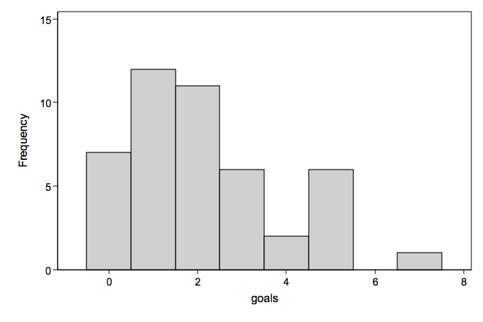
Number goals displayed as a connected line graph
Observed number of goals overlayed with a Poisson distribution
Observed number of goals overlayed with a negative binomial distribution
Exposure
Count models need some sort of mechanism to deal with the fact that counts can be made over different observation periods. For example, the number of accidents are recorded for 50 different intersections. However, the number of vehicles that pass through the intersections can vary greatly. Fifteen accidents for 30,000 vehicles is very different from 15 accidents for 1,500 vehicles. Count models account for these differences by including the log of the exposure variable in model with coefficient constrained to be one.
The use of exposure is superior in many instances to analyzing rates as response variables because it makes use of the correct probability distributions. It should be noted that exposure is used to adjust counts on the response variable and that it is possible to various kinds of rates, indexes or per capita measures as predictors.
Deaths
The response variable is the number of deaths recorded at each of five different age-group and two smoker categories. The difference in the number of patient years will be accounted for with an exposure variable pyears. Below, note that rows 1 and 10 have almost identical numbers of deaths but have very different values for patient years.
   agecat     smokes     deaths     pyears
        1          1         32     52,407
        2          1        104     43,248
        3          1        206     28,612
        4          1        186     12,663
        5          1        102      5,317
        1          0          2     18,790
        2          0         12     10,673
        3          0         28      5,710
        4          0         28      2,585
        5          0         31      1,462

    variable |         N      mean  variance       min       max
-------------+--------------------------------------------------
      deaths |        10      73.1  5390.767         2       206
      pyears |        10   18146.7  3.16e+08      1462     52407
----------------------------------------------------------------
The predictor variables are four age-group dummy variables and a dummy variable to indicate smokers.
These data can be analyzed with either a Poisson regression model or a negative binomial regression model.
     ll    df    BIC     model
 -33.60015  6   81.0158  poisson
 -33.60014  7   83.3184  negative binomial
There is not much difference between the two models based on the log-likelihood and the BIC but the Poisson model has a slightly better BIC.
Poisson regression                                Number of obs   =         10
                                                  LR chi2(5)      =     922.93
                                                  Prob > chi2     =     0.0000
Log likelihood = -33.600153                       Pseudo R2       =     0.9321

------------------------------------------------------------------------------
      deaths |      Coef.   Std. Err.      z    P>|z|     [95% Conf. Interval]
-------------+----------------------------------------------------------------
      smokes |   .3545356   .1073741     3.30   0.001     .1440862     .564985
          a2 |   1.484007   .1951034     7.61   0.000     1.101611    1.866403
          a3 |   2.627505   .1837273    14.30   0.000     2.267406    2.987604
          a4 |   3.350493   .1847992    18.13   0.000     2.988293    3.712693
          a5 |   3.700096   .1922195    19.25   0.000     3.323353     4.07684
       _cons |  -7.919326   .1917618   -41.30   0.000    -8.295172   -7.543479
      pyears | (exposure)
------------------------------------------------------------------------------
Zero-inflated Models
Zero-inflated models attempt to account for excess zeros, i.e., there is thought to be two kinds of zeros, “true zeros” and excess zeros. Zero-inflated models estimate two equations, one for the count model and one for the excess zero’s.
Fishing Example
Somehow, it seems very appropriate to discuss fish and Poisson in the same example.
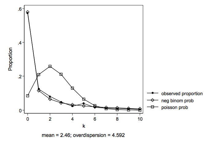
Response variable: count — the number of fish caught by visitors to a state park
Predictors: child — number of children in group camper — camping one or more nights during stay (0/1) persons — number of people in group
Child is also used as the predictor of the inflated-zeros
In our example “true zeros” are obtained from people who fish but do not catch anything. The excess zeros come from those who do not fish at all. Separate equations are used to predict each kind of zero.
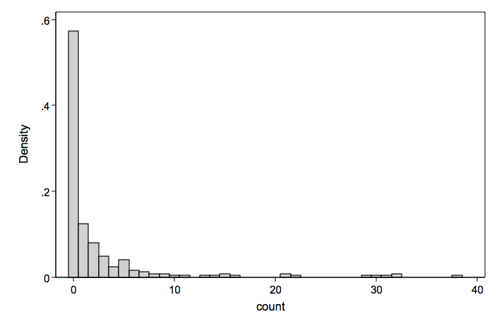
We will look at two count models and two zero-inflated models and an OLS regression for comparison.
    ll    df     BIC    model
 -749.3503 4  1520.754  ols
 -645.2568 4  1312.567  poisson
 -391.0271 5   809.621  negative binomial
 -561.5176 6  1156.116  zero-inflated poisson
 -384.8586 7   808.311  zero-inflated negative binomial
The results for the zero-inflated negative binomial are given below. Note this model is only marginally better than the ordinary negative binomial model and the Vuong test is not significant but the data were clearly generated by a process that leads to inflated zeros.
Zero-inflated negative binomial regression        Number of obs   =        248
                                                  Nonzero obs     =        106
                                                  Zero obs        =        142

Inflation model = logit                           LR chi2(3)      =      69.88
Log likelihood  = -384.8586                       Prob > chi2     =     0.0000

------------------------------------------------------------------------------
             |      Coef.   Std. Err.      z    P>|z|     [95% Conf. Interval]
-------------+----------------------------------------------------------------
count        |
       child |  -1.017093   .2734393    -3.72   0.000    -1.553025   -.4811623
      camper |   .4953317   .2320177     2.13   0.033     .0405854     .950078
     persons |   .9412857   .1142745     8.24   0.000     .7173118     1.16526
       _cons |  -1.440209   .3237543    -4.45   0.000    -2.074756   -.8056624
-------------+----------------------------------------------------------------
inflate      |
       child |   2.857134   .7912044     3.61   0.000     1.306402    4.407866
       _cons |  -4.155515   1.358571    -3.06   0.002    -6.818266   -1.492765
-------------+----------------------------------------------------------------
    /lnalpha |   .5080559   .1945664     2.61   0.009     .1267128     .889399
-------------+----------------------------------------------------------------
       alpha |   1.662057   .3233804                      1.135091    2.433667
------------------------------------------------------------------------------
Likelihood-ratio test of alpha=0: chibar2(01) =   353.32 Pr>=chibar2 =  0.0000
Vuong test of zinb vs. standard negative binomial: z =     1.29  Pr>z = 0.0981
Here are the results from the several of the other models that we can look at the differences in the output.
OLS regression

      Source |       SS       df       MS              Number of obs =     248
-------------+------------------------------           F(  3,   244) =   31.67
       Model |  2381.37932     3  793.793107           Prob > F      =  0.0000
    Residual |  6116.21745   244   25.066465           R-squared     =  0.2802
-------------+------------------------------           Adj R-squared =  0.2714
       Total |  8497.59677   247  34.4032258           Root MSE      =  5.0066

------------------------------------------------------------------------------
       count |      Coef.   Std. Err.      t    P>|t|     [95% Conf. Interval]
-------------+----------------------------------------------------------------
       child |   -3.66316   .4517096    -8.11   0.000    -4.552908   -2.773412
      camper |   1.803715   .6462559     2.79   0.006     .5307624    3.076667
     persons |   2.958617   .3471834     8.52   0.000     2.274758    3.642476
       _cons |  -3.513368    .911917    -3.85   0.000    -5.309602   -1.717134
------------------------------------------------------------------------------

Poisson regression

Poisson regression                                Number of obs   =        248
                                                  LR chi2(3)      =     825.76
                                                  Prob > chi2     =     0.0000
Log likelihood = -645.25676                       Pseudo R2       =     0.3902

------------------------------------------------------------------------------
       count |      Coef.   Std. Err.      z    P>|z|     [95% Conf. Interval]
-------------+----------------------------------------------------------------
       child |  -1.435991   .0817147   -17.57   0.000    -1.596149   -1.275834
      camper |   .6581591   .0928267     7.09   0.000     .4762221     .840096
     persons |   .8921543   .0412052    21.65   0.000     .8113936     .972915
       _cons |  -1.406989   .1512168    -9.30   0.000    -1.703369    -1.11061
------------------------------------------------------------------------------

Negative binomial regression

Negative binomial regression                      Number of obs   =        248
                                                  LR chi2(3)      =      94.97
Dispersion     = mean                             Prob > chi2     =     0.0000
Log likelihood = -391.02712                       Pseudo R2       =     0.1083

------------------------------------------------------------------------------
       count |      Coef.   Std. Err.      z    P>|z|     [95% Conf. Interval]
-------------+----------------------------------------------------------------
       child |  -1.663023   .1952636    -8.52   0.000    -2.045732   -1.280313
      camper |   .5581623   .2323451     2.40   0.016     .1027743     1.01355
     persons |   .9721464   .1223069     7.95   0.000     .7324293    1.211864
       _cons |  -1.462463    .334303    -4.37   0.000    -2.117685   -.8072411
-------------+----------------------------------------------------------------
    /lnalpha |   .7456885   .1585742                      .4348888    1.056488
-------------+----------------------------------------------------------------
       alpha |   2.107892   .3342573                      1.544791    2.876253
------------------------------------------------------------------------------
Likelihood-ratio test of alpha=0:  chibar2(01) =  508.46 Prob>=chibar2 = 0.000
Days Absent From School
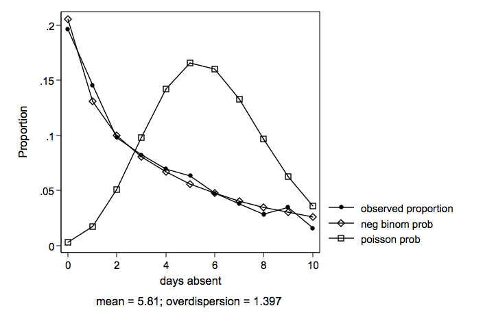
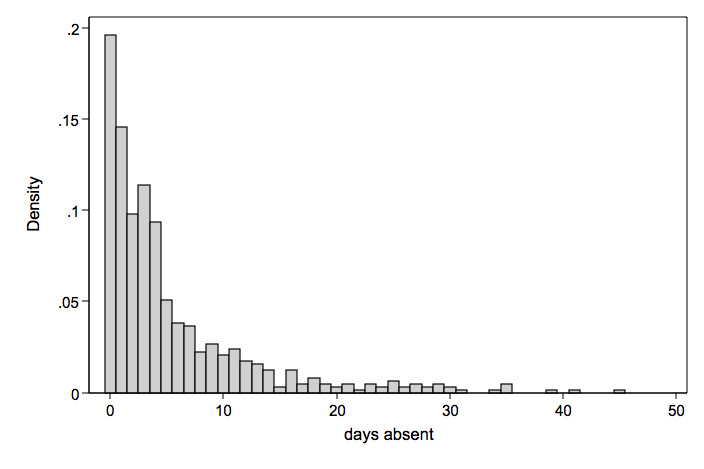
Days absent from school during one school year (mean = 5.81 variance = 55.49)
Predictors of the count variable are female, school and reading.
Several variables were tried as predictors of excess zeros for zero-inflated models. The large number of zeros in the data might seem to suggest some type of zero-inflated model. However, the zero-inflated models were not used for both empirical reasons and because there did not seem to be a reasonable way explain what kind of a process would generate excess zeros in days absent.
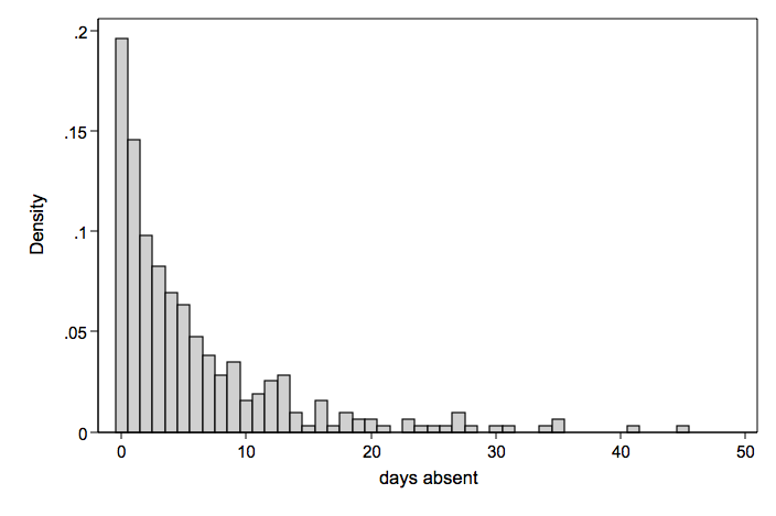
Histogram of days absent by school.
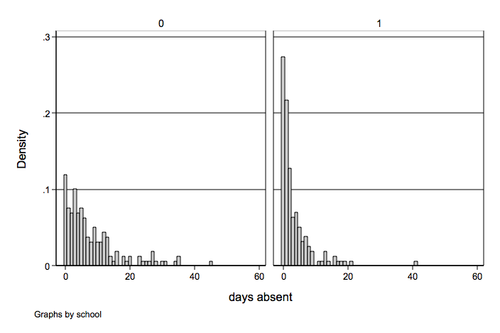
We will look at five different models, two count models, two zero-inflated count model and an ols regression thrown in for good measure.
    ll    df     BIC    model
-1060.365  4  2143.75   ols regression
-1435.846  3  2894.72   poisson
 -867.240  4  1763.26   negative binomial
-1278.182  5  2590.90   zero-inflated poisson
 -867.200  6  1774.69   zero-inflated negative binomial
Both the negative binomial and the zero-inflated negative binomial are very close in log likelihoods and BIC’s, there’s a slight edge to the straight negative binomial due to having fewer degrees of freedom.
Negative binomial regression                      Number of obs   =        316
                                                  LR chi2(2)      =      44.02
Dispersion     = mean                             Prob > chi2     =     0.0000
Log likelihood = -869.23382                       Pseudo R2       =     0.0247

------------------------------------------------------------------------------
     daysabs |      Coef.   Std. Err.      z    P>|z|     [95% Conf. Interval]
-------------+----------------------------------------------------------------
      female |   .3366034    .132156     2.55   0.011     .0775823    .5956244
      school |  -.8628592   .1323017    -6.52   0.000    -1.122166   -.6035526
       _cons |   2.776001   .2142417    12.96   0.000     2.356094    3.195907
-------------+----------------------------------------------------------------
    /lnalpha |   .1568369   .0986426                      -.036499    .3501728
-------------+----------------------------------------------------------------
       alpha |   1.169805   .1153925                      .9641591    1.419313
------------------------------------------------------------------------------
Likelihood-ratio test of alpha=0:  chibar2(01) = 1152.21 Prob>=chibar2 = 0.000
Zero-truncated Models
There are a number of interesting situations in which the count variable cannot take on the value zero.
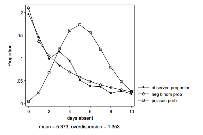
Take for example the response variable length of hospital stay (mean = 5.37 variance = 49.24). The predictor variables are age, hmo and died (died before discharge). Note that there are no zero counts in the data.
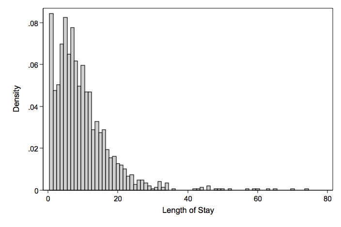
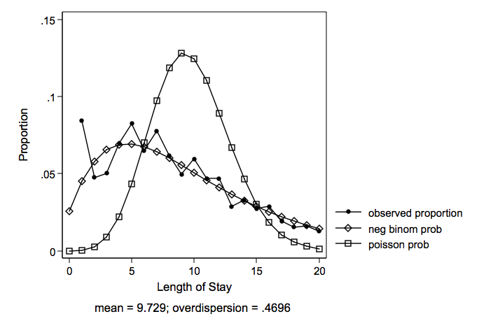
Note that both Poisson and negative binomial predict a probability for zero length of hospital stay. The negative binomial provides a closer fit to the observed than does the Poisson.
    ll     df      BIC   model
-6908.799   4  13846.83  zero-truncated poisson
-4755.28    5   9547.10  zero-truncated negative binomial
The results for the zero-truncated negative binomial are given below.
Zero-truncated negative binomial regression       Number of obs   =       1493
                                                  LR chi2(3)      =      31.14
Dispersion     = mean                             Prob > chi2     =     0.0000
Log likelihood = -4755.2796                       Pseudo R2       =     0.0033

------------------------------------------------------------------------------
        stay |      Coef.   Std. Err.      z    P>|z|     [95% Conf. Interval]
-------------+----------------------------------------------------------------
         age |  -.0156929    .013107    -1.20   0.231    -.0413822    .0099964
         hmo |  -.1470576   .0592161    -2.48   0.013     -.263119   -.0309962
        died |  -.2177714   .0461605    -4.72   0.000    -.3082442   -.1272985
       _cons |   2.408328    .071982    33.46   0.000     2.267245     2.54941
-------------+----------------------------------------------------------------
    /lnalpha |  -.5686389   .0551506                     -.6767321   -.4605457
-------------+----------------------------------------------------------------
       alpha |   .5662957   .0312316                      .5082753    .6309393
------------------------------------------------------------------------------
Likelihood-ratio test of alpha=0:  chibar2(01) = 4307.04 Prob>=chibar2 = 0.000
Hurdle Models
A hurdle model is a modified count model in which there are two processes, one generating the zeros and one generating the positive values. The two models are not constrained to be the same. The concept underlying the hurdle model is that a binomial probability model governs the binary outcome of whether a count variable has a zero or a positive value. If the value is positive, the “hurdle is crossed,” and the conditional distribution of the positive values is governed by a zero-truncated count model.
We will illustrate this model using artificially generated data with response variable y and predictors x1 and x2.
         y |      Freq.
------------+---------------
          0 |        315
          1 |        123
          2 |        138
          3 |        117
          4 |         88
          5 |         60
          6 |         35
          7 |         23
          8 |         24
          9 |         19
         10 |         16
         11 |         11
         12 |         10
         13 |          5
         14 |          1
         15 |          4
         16 |          1
         19 |          2
         21 |          2
         22 |          2
         26 |          1
         32 |          2
         34 |          1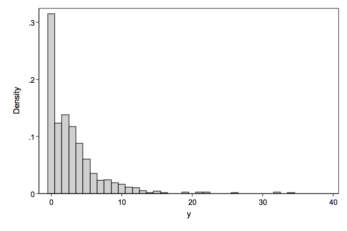
Since the count part of the model was generated using a random Poisson generator, we will look at three different Poisson based models.
    ll     df        BIC   model
-2133.079   3     4286.881 poisson
-1748.863   6     3539.173 zero-inflated poisson
-1730.438   6     3502.322 poisson-logit hurdle
The Poisson-logit hurdle model is clearly the best choice here. The results for this model are given below
Poisson-Logit Hurdle Regression                   Number of obs   =       1000
                                                  Wald chi2(2)    =     187.13
Log likelihood = -1730.4377                       Prob > chi2     =     0.0000

------------------------------------------------------------------------------
             |      Coef.   Std. Err.      z    P>|z|     [95% Conf. Interval]
-------------+----------------------------------------------------------------
logit        |
          x1 |   1.494141   .1092238    13.68   0.000     1.280067    1.708216
          x2 |   .0637035    .086461     0.74   0.461     -.105757     .233164
       _cons |   .9951839   .0855003    11.64   0.000     .8276064    1.162761
-------------+----------------------------------------------------------------
poisson      |
          x1 |   .1732047   .0226329     7.65   0.000      .128845    .2175644
          x2 |   .7216143   .0198055    36.44   0.000     .6827963    .7604324
       _cons |   1.009172   .0284237    35.50   0.000     .9534629    1.064882
------------------------------------------------------------------------------
Days Absent Clustered in Schools
We will take another look at days absent (mean = 5.37 variance = 49.24), this time obtained from 12 schools with about 50 students per school. The predictors are gender and reading. Any count model will need to account for the lack of independence within schools.
We have a number of options for analyzing these data. We can use standard poisson with cluster robust standard errors to account for within school association. Or we can use one of the random-effects models for poisson or negative binomial. These are random intercept only models.
    ll    df     BIC    model
-2938.653  3  5896.653  poisson with cluster robust standard errors
-1718.321  4  3462.437  negative binomial with cluster robust standard errors
-2718.767  4  5463.33   random-effects poisson w/ gaussian random effects
-2718.864  4  5463.523  random-effects poisson w/ gamma random effects
-1696.797  5  3425.838  random-effects negative binomial w/ beta random effects
The random-effects negative binomial has the best log likelihood and BIC. The results of the model are given below.
Random-effects negative binomial regression     Number of obs      =       632
Group variable (i): sid                         Number of groups   =        12

Random effects u_i ~ Beta                       Obs per group: min =        51
                                                               avg =      52.7
                                                               max =        53

                                                Wald chi2(2)       =     36.14
Log likelihood  = -1696.7966                    Prob > chi2        =    0.0000

------------------------------------------------------------------------------
     daysabs |      Coef.   Std. Err.      z    P>|z|     [95% Conf. Interval]
-------------+----------------------------------------------------------------
      female |   .3587537   .0788313     4.55   0.000     .2042472    .5132602
     reading |  -.0102389   .0022909    -4.47   0.000    -.0147289   -.0057489
       _cons |   .1944149    .131354     1.48   0.139    -.0630343     .451864
-------------+----------------------------------------------------------------
       /ln_r |   2.260673   .4859689                      1.308192    3.213155
       /ln_s |   3.922436   .5105199                      2.921835    4.923037
-------------+----------------------------------------------------------------
           r |   9.589543    4.66022                      3.699478    24.85738
           s |   50.52336   25.79318                      18.57535    137.4193
------------------------------------------------------------------------------
Likelihood-ratio test vs. pooled: chibar2(01) =    32.25 Prob>=chibar2 = 0.000
Summary of Count Regression Models
- Poisson regression model
- Negative binomial regression model
- Zero-inflated poisson model
- Zero-inflated negative binomial model
- Zero-truncated poisson model
- Zero-truncated negative binomial model
- Hurdle models
- Random-effects count models
Some Stata Specific Information
Here are the Stata commands for selected models shown above:
poisson regression with exposure, deaths
(also see DAE page):

. poisson deaths smokes a2 a3 a4 a5, exposure(pyears)

zero-inflated negative binomial, fish
(also see DAE page):

. zinb count child camper persons, inflate(child) vuong zip

negative binomial regression, days absent
(also see DAE page):

. nbreg daysabs female school

Zero-truncated negative binomial regression, length of hosptial stay
(also see DAE page):

. ztnb stay age hmo died

Poisson-Logit Hurdle Regression, artifical data

. hplogit y x1 x2

negative binomial regression with cluster robust standard errors, days absent:

. nbreg daysabs female reading, cluster(sid)

random effects negative binomial, days absent:

. xtnbreg daysabs female reading, i(sid)
References Here are some places to read more about regression models with count data.
Agresti, A. (2001) Categorical Data Analysis (2nd ed). New York: Wiley.
Agresti, A. (1996) An Introduction to Categorical Data Analysis. New York: Wiley.
Long, S. J. (1997) Regression Models for Categorical and Limited Dependent Variables. Thousand Oaks, CA: SAGE Publications, Inc.
Long, S. J. & Freese, J. (2001) Regression Models for Categorical Dependent Variables using Stata. College Station, TX: Stata Press.
